Ch 9 Unsupervised Learning Stephen Marsland Machine Learning

Ch. 9 Unsupervised Learning Stephen Marsland, Machine Learning: An Algorithmic Perspective. CRC 2009 based on slides from Stephen Marsland some slides from the Internet Collected and modified by Longin Jan Latecki Temple University latecki@temple. edu 159. 302 3. 1 Stephen Marsland

Introduction Suppose we don’t have good training data Hard and boring to generate targets Don’t always know target values Biologically implausible to have targets? Two cases: Know when we’ve got it right No external information at all 159. 302 3. 2 Stephen Marsland

Unsupervised Learning We have no external error information No task-specific error criterion Generate internal error Must be general Usual method is to cluster data together according to activation of neurons Competitive learning 159. 302 3. 3 Stephen Marsland

Competitive Learning Set of neurons compete to fire Neuron that ‘best matches’ the input (has the highest activation) fires Winner-take-all Neurons ‘specialise’ to recognise some input Grandmother cells 159. 302 3. 4 Stephen Marsland

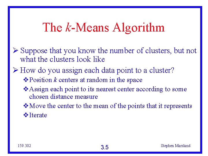
The k-Means Algorithm Suppose that you know the number of clusters, but not what the clusters look like How do you assign each data point to a cluster? Position k centers at random in the space Assign each point to its nearest center according to some chosen distance measure Move the center to the mean of the points that it represents Iterate 159. 302 3. 5 Stephen Marsland

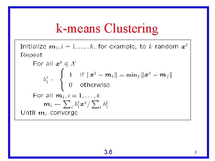
k-means Clustering 3. 6 6

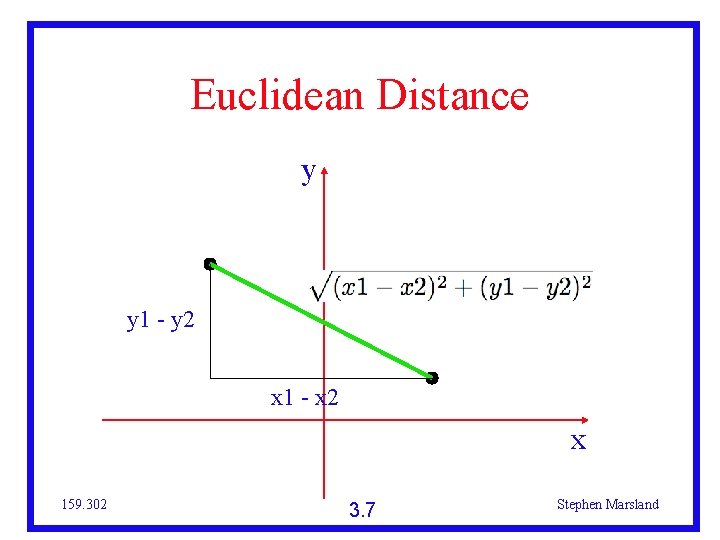
Euclidean Distance y y 1 - y 2 x 1 - x 2 x 159. 302 3. 7 Stephen Marsland

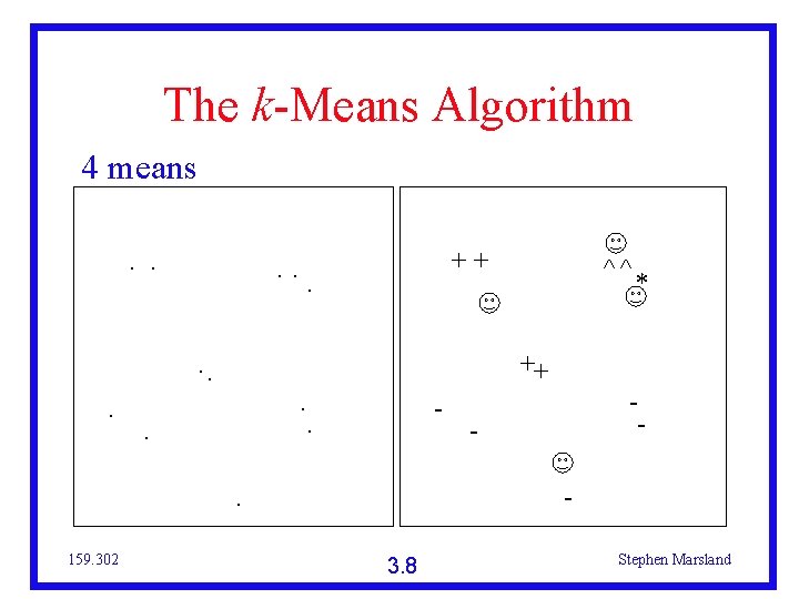
The k-Means Algorithm 4 means. . ++. . - . * - - . 159. 302 ^^ 3. 8 Stephen Marsland

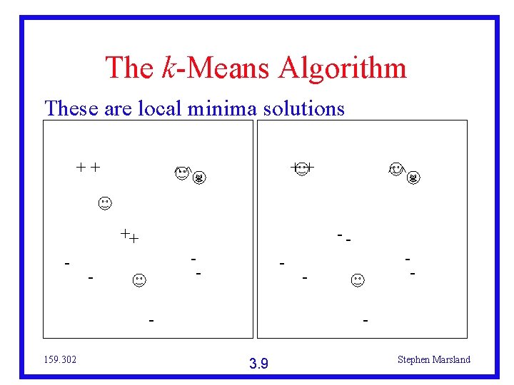
The k-Means Algorithm These are local minima solutions ++ ^^ ++ - ++ * -- - 159. 302 ^^ * - - 3. 9 Stephen Marsland

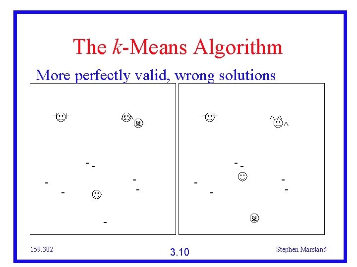
The k-Means Algorithm More perfectly valid, wrong solutions ++ ^^ -- - ++ * -- - 159. 302 ^^ ^ - * 3. 10 Stephen Marsland

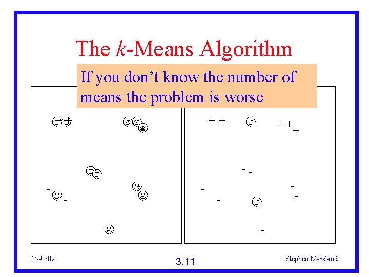
The k-Means Algorithm If you don’t know the number of means the problem is worse ++ ^^ -- - ++ * -- - 159. 302 ++ + - - 3. 11 Stephen Marsland

The k-Means Algorithm One solution is to run the algorithm for many values of k Pick the one with lowest error Up to overfitting Run the algorithm from many starting points Avoids local minima? What about noise? Median instead of mean? 159. 302 3. 12 Stephen Marsland

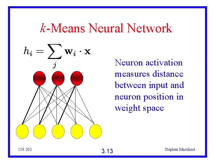
k-Means Neural Network Neuron activation measures distance between input and neuron position in weight space 159. 302 3. 13 Stephen Marsland

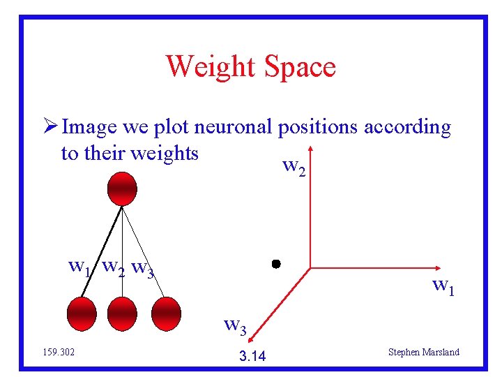
Weight Space Image we plot neuronal positions according to their weights w 2 w 1 w 2 w 3 w 1 w 3 159. 302 3. 14 Stephen Marsland

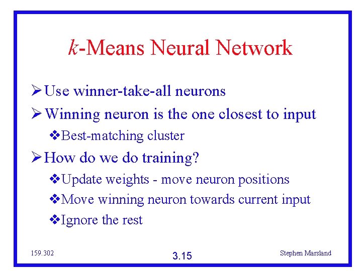
k-Means Neural Network Use winner-take-all neurons Winning neuron is the one closest to input Best-matching cluster How do we do training? Update weights - move neuron positions Move winning neuron towards current input Ignore the rest 159. 302 3. 15 Stephen Marsland

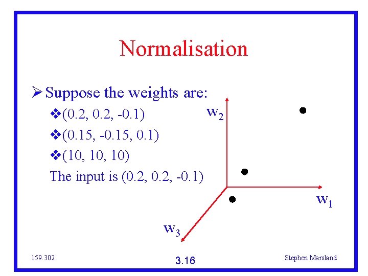
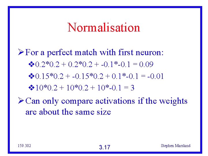
Normalisation Suppose the weights are: w 2 (0. 2, -0. 1) (0. 15, -0. 15, 0. 1) (10, 10) The input is (0. 2, -0. 1) w 1 w 3 159. 302 3. 16 Stephen Marsland

Normalisation For a perfect match with first neuron: 0. 2*0. 2 + -0. 1*-0. 1 = 0. 09 0. 15*0. 2 + -0. 15*0. 2 + 0. 1*-0. 1 = -0. 01 10*0. 2 + 10*-0. 1 = 3 Can only compare activations if the weights are about the same size 159. 302 3. 17 Stephen Marsland

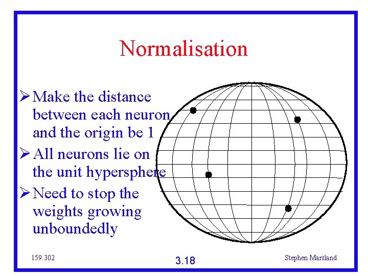
Normalisation Make the distance between each neuron and the origin be 1 All neurons lie on the unit hypersphere Need to stop the weights growing unboundedly 159. 302 3. 18 Stephen Marsland

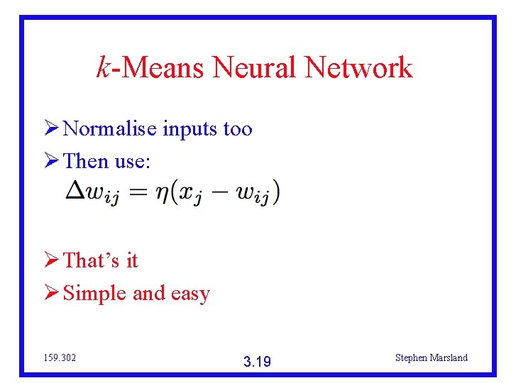
k-Means Neural Network Normalise inputs too Then use: That’s it Simple and easy 159. 302 3. 19 Stephen Marsland

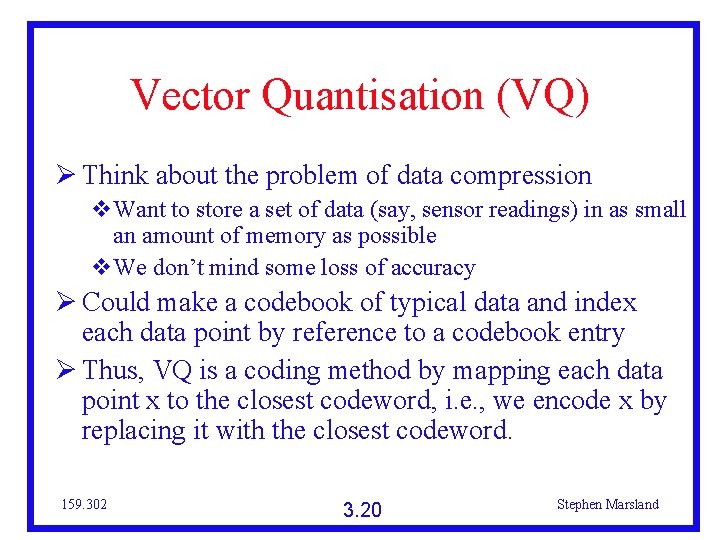
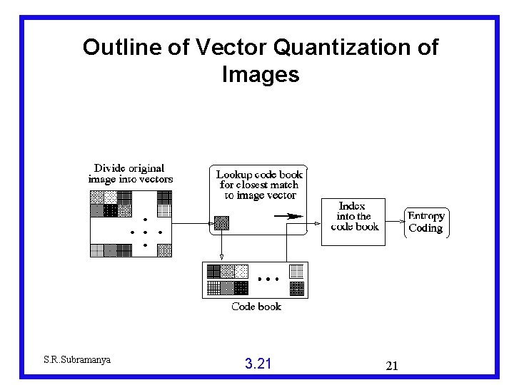
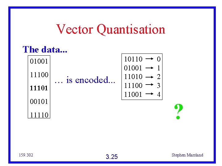
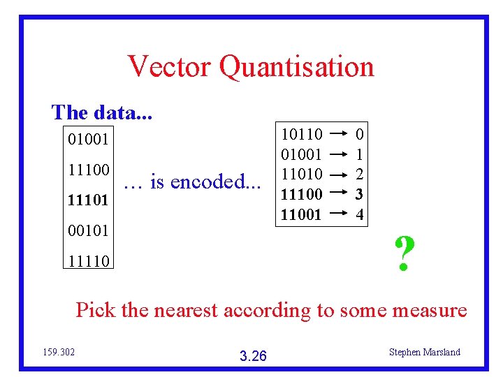
Vector Quantisation (VQ) Think about the problem of data compression Want to store a set of data (say, sensor readings) in as small an amount of memory as possible We don’t mind some loss of accuracy Could make a codebook of typical data and index each data point by reference to a codebook entry Thus, VQ is a coding method by mapping each data point x to the closest codeword, i. e. , we encode x by replacing it with the closest codeword. 159. 302 3. 20 Stephen Marsland

Outline of Vector Quantization of Images S. R. Subramanya 3. 21 21

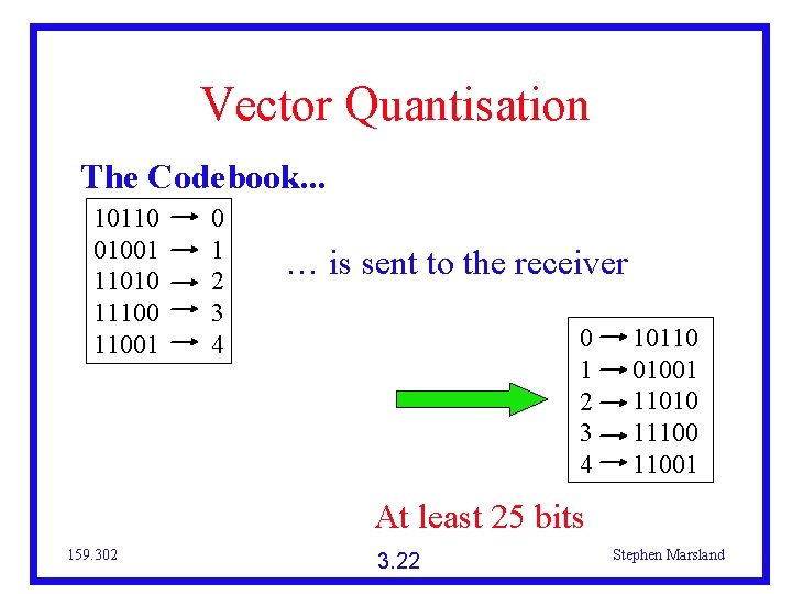
Vector Quantisation The Codebook. . . 10110 01001 11010 111001 0 1 2 3 4 … is sent to the receiver 0 1 2 3 4 10110 01001 11010 111001 At least 25 bits 159. 302 3. 22 Stephen Marsland

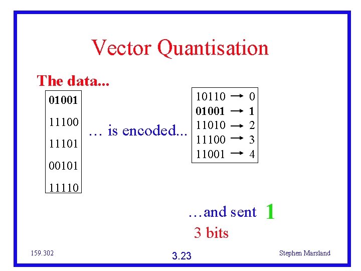
Vector Quantisation The data. . . 01001 11100 11101 … is encoded. . . 00101 10110 01001 11010 111001 0 1 2 3 4 11110 …and sent 3 bits 159. 302 3. 23 1 Stephen Marsland

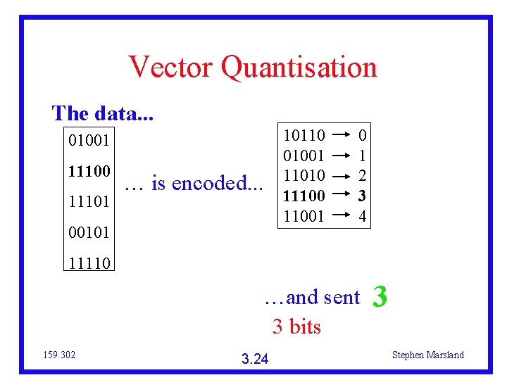
Vector Quantisation The data. . . 01001 11100 11101 … is encoded. . . 00101 10110 01001 11010 111001 0 1 2 3 4 11110 …and sent 3 bits 159. 302 3. 24 3 Stephen Marsland

Vector Quantisation The data. . . 01001 11100 11101 … is encoded. . . 00101 0 1 2 3 4 ? 11110 159. 302 10110 01001 11010 111001 3. 25 Stephen Marsland

Vector Quantisation The data. . . 01001 11100 11101 … is encoded. . . 00101 10110 01001 11010 111001 0 1 2 3 4 ? 11110 Pick the nearest according to some measure 159. 302 3. 26 Stephen Marsland

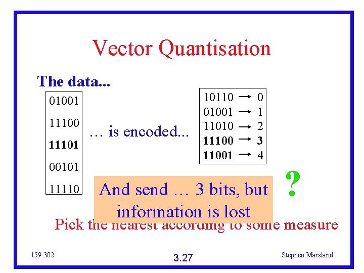
Vector Quantisation The data. . . 01001 11100 11101 … is encoded. . . 00101 11110 10110 01001 11010 111001 0 1 2 3 4 And send … 3 bits, but information is lost ? Pick the nearest according to some measure 159. 302 3. 27 Stephen Marsland

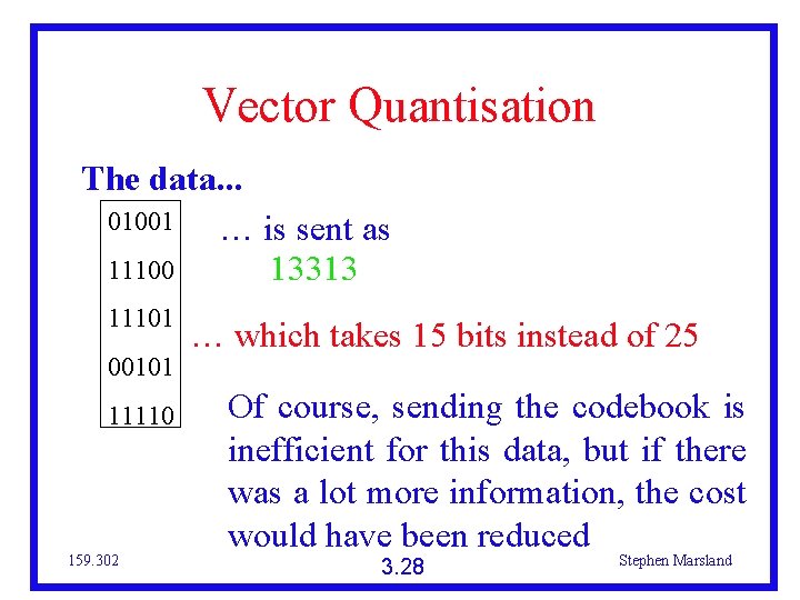
Vector Quantisation The data. . . 01001 … is sent as 11100 13313 11101 00101 11110 159. 302 … which takes 15 bits instead of 25 Of course, sending the codebook is inefficient for this data, but if there was a lot more information, the cost would have been reduced 3. 28 Stephen Marsland

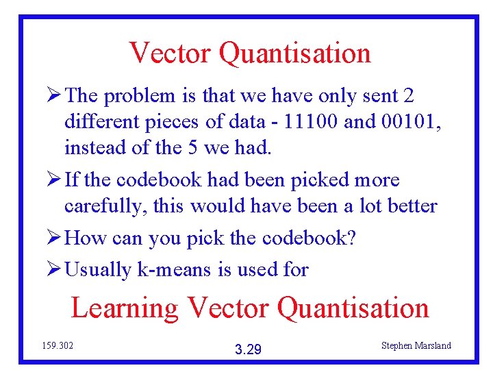
Vector Quantisation The problem is that we have only sent 2 different pieces of data - 11100 and 00101, instead of the 5 we had. If the codebook had been picked more carefully, this would have been a lot better How can you pick the codebook? Usually k-means is used for Learning Vector Quantisation 159. 302 3. 29 Stephen Marsland

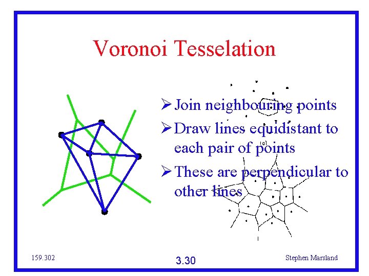
Voronoi Tesselation Join neighbouring points Draw lines equidistant to each pair of points These are perpendicular to other lines 159. 302 3. 30 Stephen Marsland

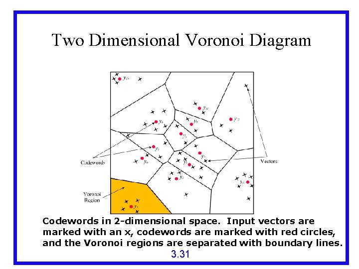
Two Dimensional Voronoi Diagram Codewords in 2 -dimensional space. Input vectors are marked with an x, codewords are marked with red circles, and the Voronoi regions are separated with boundary lines. 3. 31

Self Organizing Maps Self-organizing maps (SOMs) are a data visualization technique invented by Professor Teuvo Kohonen Also called Kohonen Networks, Competitive Learning, Winner-Take-All Learning Generally reduces the dimensions of data through the use of self-organizing neural networks Useful for data visualization; humans cannot visualize high dimensional data so this is often a useful technique to make sense of large data sets 3. 32

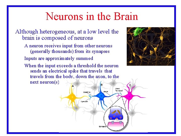
Neurons in the Brain Although heterogeneous, at a low level the brain is composed of neurons A neuron receives input from other neurons (generally thousands) from its synapses Inputs are approximately summed When the input exceeds a threshold the neuron sends an electrical spike that travels from the body, down the axon, to the next neuron(s) 3. 33

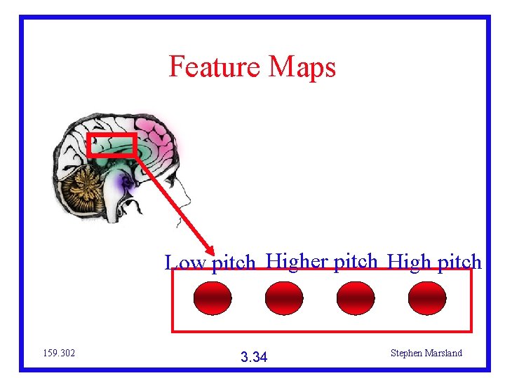
Feature Maps Low pitch Higher pitch High pitch 159. 302 3. 34 Stephen Marsland

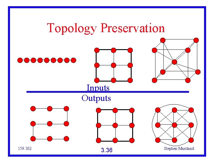
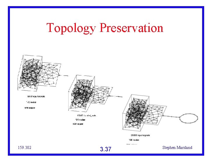
Feature Maps Sounds that are similar (‘close together’) excite neurons that are near to each other Sounds that are very different excite neurons that are a long way off This is known as topology preservation The ordering of the inputs is preserved If possible (perfectly topology-preserving) 159. 302 3. 35 Stephen Marsland

Topology Preservation Inputs Outputs 159. 302 3. 36 Stephen Marsland

Topology Preservation 159. 302 3. 37 Stephen Marsland

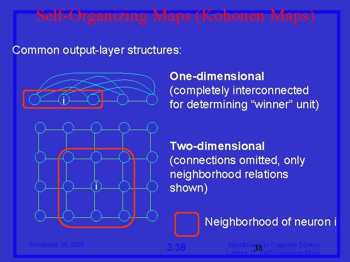
Self-Organizing Maps (Kohonen Maps) Common output-layer structures: One-dimensional (completely interconnected for determining “winner” unit) i i Two-dimensional (connections omitted, only neighborhood relations shown) Neighborhood of neuron i November 24, 2009 3. 38 Introduction to Cognitive Science 38 Lecture 21: Self-Organizing Maps

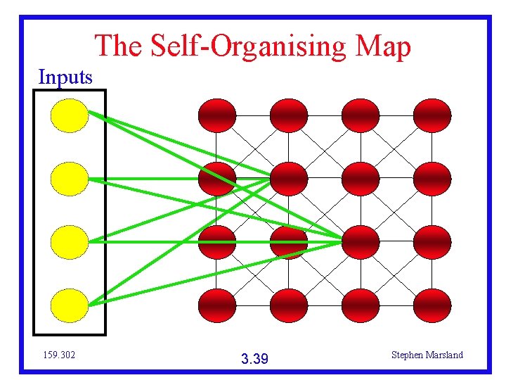
The Self-Organising Map Inputs 159. 302 3. 39 Stephen Marsland

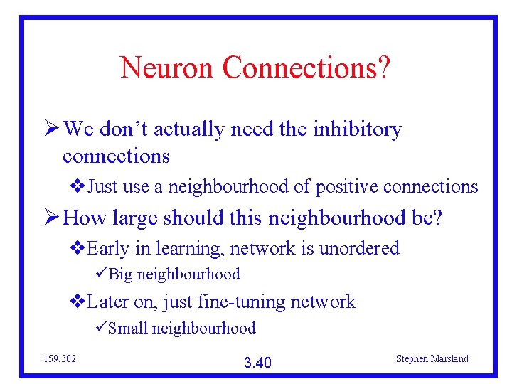
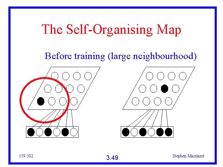
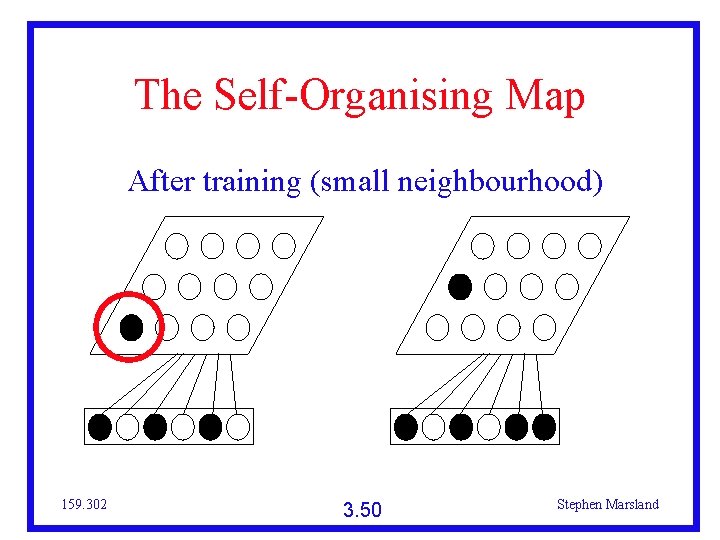
Neuron Connections? We don’t actually need the inhibitory connections Just use a neighbourhood of positive connections How large should this neighbourhood be? Early in learning, network is unordered Big neighbourhood Later on, just fine-tuning network Small neighbourhood 159. 302 3. 40 Stephen Marsland

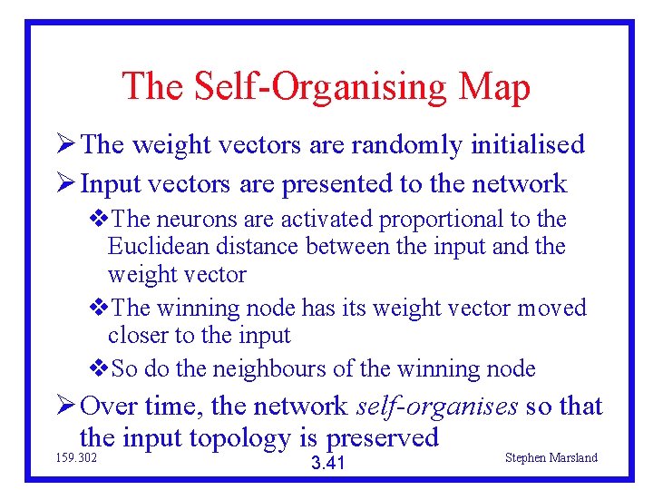
The Self-Organising Map The weight vectors are randomly initialised Input vectors are presented to the network The neurons are activated proportional to the Euclidean distance between the input and the weight vector The winning node has its weight vector moved closer to the input So do the neighbours of the winning node Over time, the network self-organises so that the input topology is preserved 159. 302 3. 41 Stephen Marsland

Self-Organisation Global ordering from local interactions Each neurons sees its neighbours The whole network becomes ordered Understanding self-organisation is part of complexity science Appears all over the place 159. 302 3. 42 Stephen Marsland

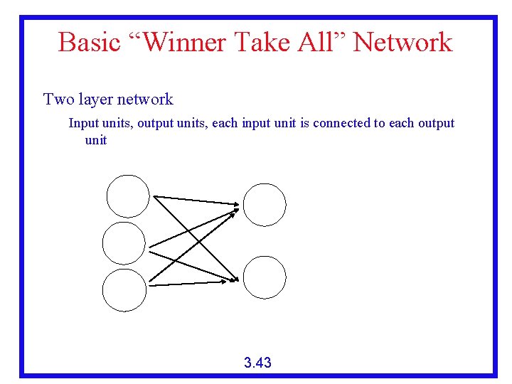
Basic “Winner Take All” Network Two layer network Input units, output units, each input unit is connected to each output unit Input Layer I 1 Output Layer O 1 I 2 I 3 O 2 Wi, j 3. 43

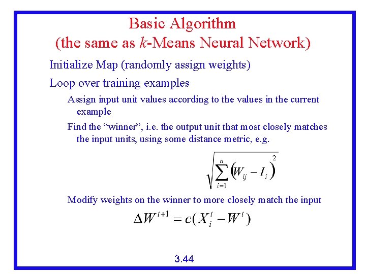
Basic Algorithm (the same as k-Means Neural Network) Initialize Map (randomly assign weights) Loop over training examples Assign input unit values according to the values in the current example Find the “winner”, i. e. the output unit that most closely matches the input units, using some distance metric, e. g. For all output units j=1 to m and input units i=1 to n Find the one that minimizes: Modify weights on the winner to more closely match the input where c is a small positive learning constant that usually decreases as the learning proceeds 3. 44

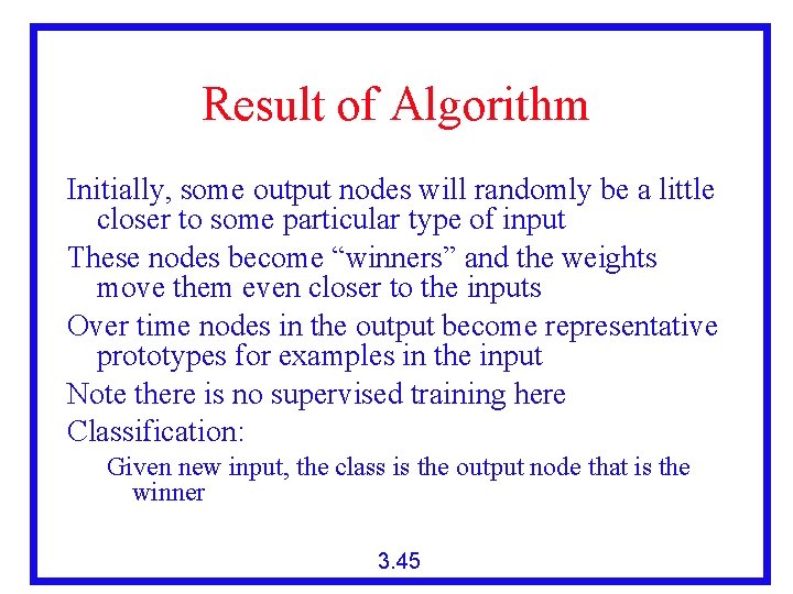
Result of Algorithm Initially, some output nodes will randomly be a little closer to some particular type of input These nodes become “winners” and the weights move them even closer to the inputs Over time nodes in the output become representative prototypes for examples in the input Note there is no supervised training here Classification: Given new input, the class is the output node that is the winner 3. 45

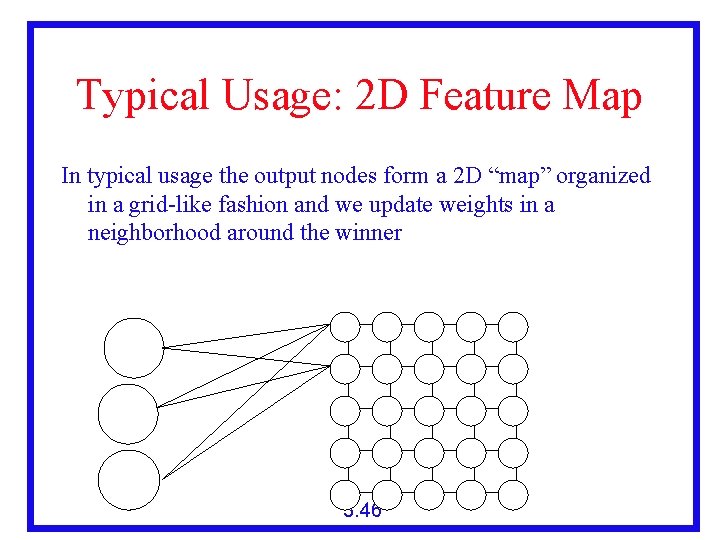
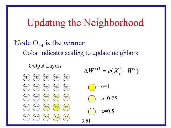
Typical Usage: 2 D Feature Map In typical usage the output nodes form a 2 D “map” organized in a grid-like fashion and we update weights in a neighborhood around the winner Output Layers Input Layer O 11 O 12 O 13 O 14 O 15 O 21 O 22 O 23 O 24 O 25 O 31 O 32 O 33 O 34 O 35 O 41 O 42 O 43 O 44 O 45 O 51 O 52 O 53 O 54 O 55 I 1 I 2 … I 3 3. 46

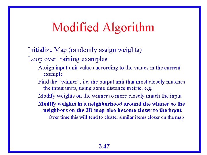
Modified Algorithm Initialize Map (randomly assign weights) Loop over training examples Assign input unit values according to the values in the current example Find the “winner”, i. e. the output unit that most closely matches the input units, using some distance metric, e. g. Modify weights on the winner to more closely match the input Modify weights in a neighborhood around the winner so the neighbors on the 2 D map also become closer to the input Over time this will tend to cluster similar items closer on the map 3. 47

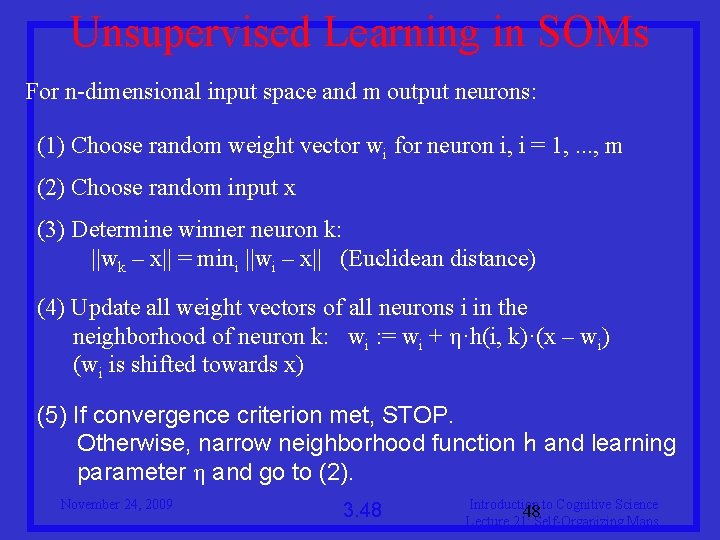
Unsupervised Learning in SOMs For n-dimensional input space and m output neurons: (1) Choose random weight vector wi for neuron i, i = 1, . . . , m (2) Choose random input x (3) Determine winner neuron k: ||wk – x|| = mini ||wi – x|| (Euclidean distance) (4) Update all weight vectors of all neurons i in the neighborhood of neuron k: wi : = wi + η·h(i, k)·(x – wi) (wi is shifted towards x) (5) If convergence criterion met, STOP. Otherwise, narrow neighborhood function h and learning parameter η and go to (2). November 24, 2009 3. 48 Introduction to Cognitive Science 48 Lecture 21: Self-Organizing Maps

The Self-Organising Map Before training (large neighbourhood) 159. 302 3. 49 Stephen Marsland

The Self-Organising Map After training (small neighbourhood) 159. 302 3. 50 Stephen Marsland

Updating the Neighborhood Node O 44 is the winner Color indicates scaling to update neighbors Output Layers O 11 O 12 O 13 O 14 O 15 O 21 O 22 O 23 O 24 O 25 c=1 O 32 O 33 O 34 O 35 c=0. 75 O 41 O 42 O 43 O 44 O 45 O 51 O 52 O 53 O 54 O 55 c=0. 5 3. 51

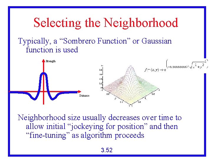
Selecting the Neighborhood Typically, a “Sombrero Function” or Gaussian function is used Strength Distance Neighborhood size usually decreases over time to allow initial “jockeying for position” and then “fine-tuning” as algorithm proceeds 3. 52

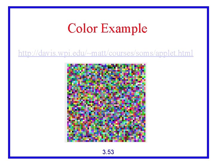
Color Example http: //davis. wpi. edu/~matt/courses/soms/applet. html 3. 53

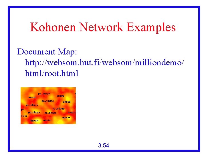
Kohonen Network Examples Document Map: http: //websom. hut. fi/websom/milliondemo/ html/root. html 3. 54

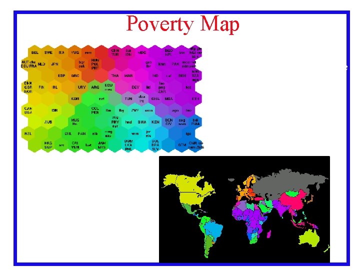
Poverty Map http: //www. cis. hut. fi/rese arch/somresearch/worldmap. html 3. 55

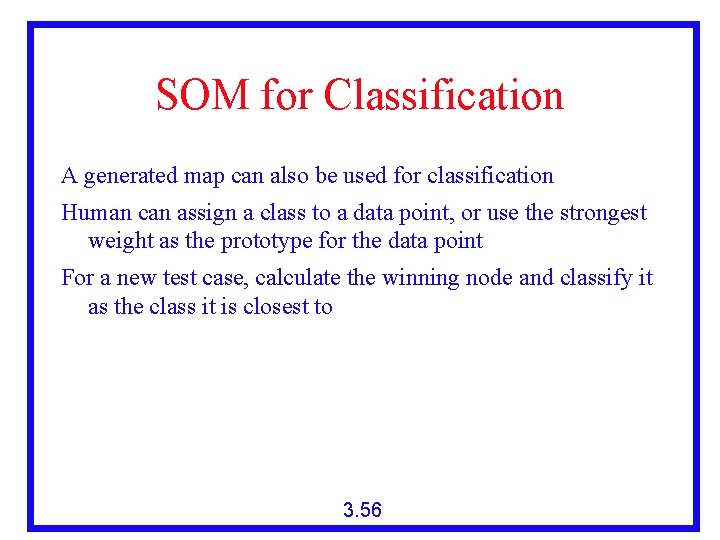
SOM for Classification A generated map can also be used for classification Human can assign a class to a data point, or use the strongest weight as the prototype for the data point For a new test case, calculate the winning node and classify it as the class it is closest to 3. 56

Network Size We have to predetermine the network size Big network Each neuron represents exact feature Not much generalisation Small network Too much generalisation No differentiation Try different sizes and pick the best 159. 302 3. 57 Stephen Marsland