Ch 9 Introduction to Convolution Neural Networks CNN

Ch. 9: Introduction to Convolution Neural Networks (CNN) and systems KH Wong ch 9. CNN. v. 0. 1. c 1

Overview • Part 1 – A 1. Theory of CNN – A 2. Feed forward details – A 2. Back propagation details • Part B: CNN Systems • Part C: CNN Tools ch 9. CNN. v. 0. 1. c 2

Introduction • Very Popular: – Toolboxes: tensorflow, cuda-convnet and caffe (user friendlier) • A high performance Classifier (multi-class) • Successful in object recognition, handwritten optical character OCR recognition, image noise removal etc. • Easy to implementation – Slow in learning – Fast in classification ch 9. CNN. v. 0. 1. c 3

Overview of this note • Prerequisite: knowledge of Fully connected Back Propagation Neural Networks (BPNN), in – http: //www. cse. cuhk. edu. hk/~khwong/www 2/cm sc 5707/5707_08_neural_net. pptx • Convolution neural networks (CNN) – Part A 2: feed forward of CNN – Part A 3: feed backward of CNN ch 9. CNN. v. 0. 1. c 4

Part A. 1 Theory of CNN Convolution Neural Networks ch 9. CNN. v. 0. 1. c 5

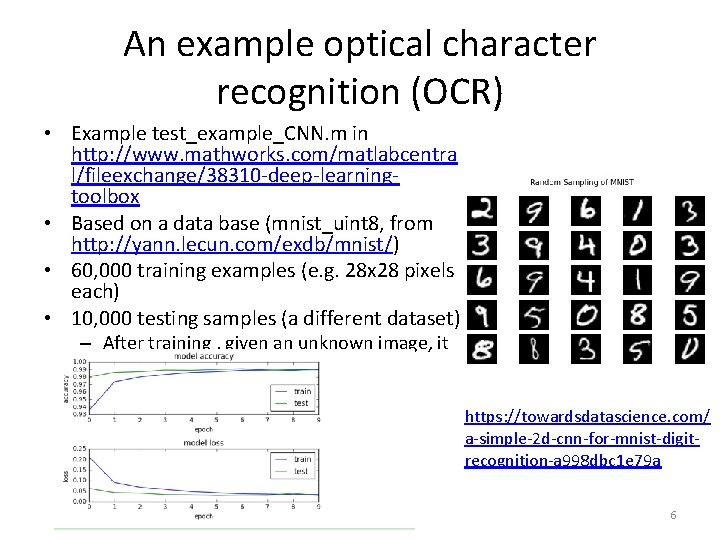
An example optical character recognition (OCR) • Example test_example_CNN. m in http: //www. mathworks. com/matlabcentra l/fileexchange/38310 -deep-learningtoolbox • Based on a data base (mnist_uint 8, from http: //yann. lecun. com/exdb/mnist/) • 60, 000 training examples (e. g. 28 x 28 pixels each) • 10, 000 testing samples (a different dataset) – After training , given an unknown image, it will tell whether it is 0, or 1 , . . , 9 etc. https: //towardsdatascience. com/ a-simple-2 d-cnn-for-mnist-digitrecognition-a 998 dbc 1 e 79 a ch 9. CNN. v. 0. 1. c 6

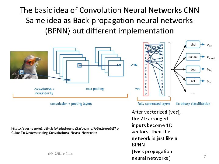
The basic idea of Convolution Neural Networks CNN Same idea as Back-propagation-neural networks (BPNN) but different implementation • https: //adeshpande 3. github. io/A-Beginner%27 s. Guide-To-Understanding-Convolutional-Neural-Networks/ ch 9. CNN. v. 0. 1. c After vectorized (vec), the 2 D arranged inputs become 1 D vectors. Then the network is just like a BPNN (Back propagation neural networks ) 7

Basic structure of CNN The convolution layer: see how to use convolution for feature identifier ch 9. CNN. v. 0. 1. c 8

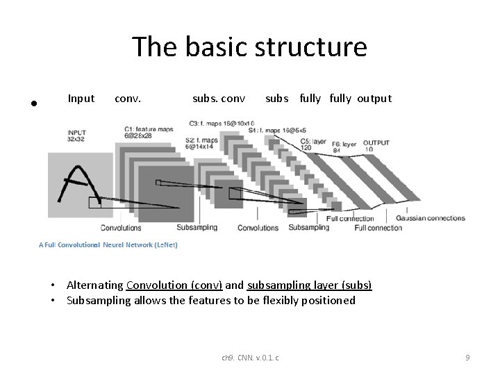
The basic structure • Input conv. subs. conv subs fully output • Alternating Convolution (conv) and subsampling layer (subs) • Subsampling allows the features to be flexibly positioned ch 9. CNN. v. 0. 1. c 9

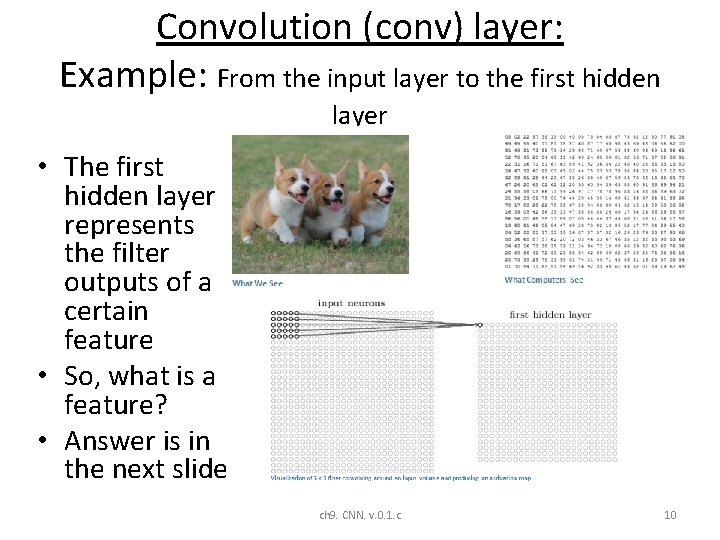
Convolution (conv) layer: Example: From the input layer to the first hidden layer • The first hidden layer represents the filter outputs of a certain feature • So, what is a feature? • Answer is in the next slide ch 9. CNN. v. 0. 1. c 10

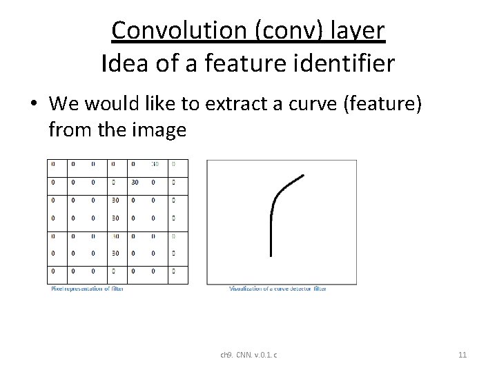
Convolution (conv) layer Idea of a feature identifier • We would like to extract a curve (feature) from the image ch 9. CNN. v. 0. 1. c 11

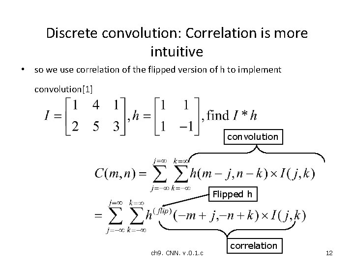
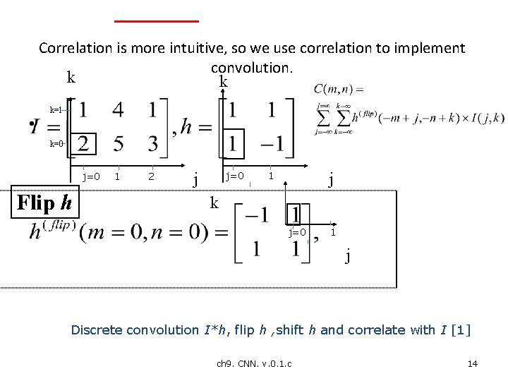
Discrete convolution: Correlation is more intuitive • so we use correlation of the flipped version of h to implement convolution[1] convolution Flipped h ch 9. CNN. v. 0. 1. c correlation 12

Matlab (octave) code for convolution • • • I=[1 4 1; 2 5 3] h=[1 1 ; 1 -1] conv 2(I, h) pause disp('It is the same as the following'); conv 2(h, I) pause disp('It is the same as the following'); xcorr 2(I, fliplr(flipud(h))) ch 9. CNN. v. 0. 1. c 13

Correlation is more intuitive, so we use correlation to implement convolution. k k • k=1 k=0 j=0 Flip h 1 2 j j=0 j 1 k j=0 1 j Discrete convolution I*h, flip h , shift h and correlate with I [1] ch 9. CNN. v. 0. 1. c 14

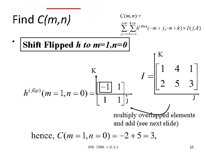
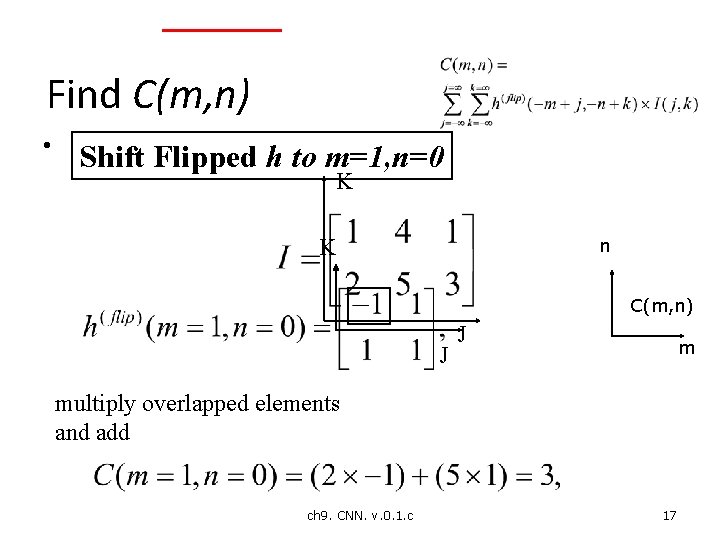
Discrete convolution I*h, flip h , shift h and correlate with I [1] k k • n j j=0 j 1 Flip h: is like this after the flip k and no shift (m=0, n=0) j Shift Flipped h to m=1, n=0 k j ch 9. CNN. v. 0. 1. c 15 C(m, n) m The trick: I(j=0, k=0) needs to multiply to h(flip)(-m+0, -n+0), since m=1, n=0, so we shift the h(flip) pattern 1 -bit to the right so we just multiply overlapped elements of I and h(flip). Similarly, we do the same for all m, n values

Find C(m, n) • Shift Flipped h to m=1, n=0 K K J J multiply overlapped elements and add (see next slide) ch 9. CNN. v. 0. 1. c 16

Find C(m, n) • Shift Flipped h to m=1, n=0 K K n C(m, n) J J m multiply overlapped elements and add ch 9. CNN. v. 0. 1. c 17

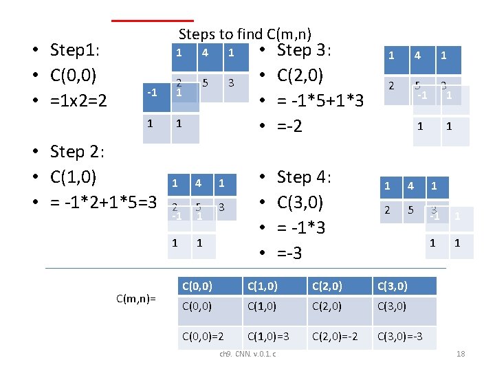
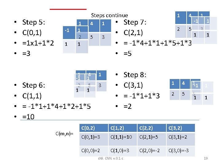
• Step 1: • C(0, 0) • =1 x 2=2 Steps to find C(m, n) 1 4 1 -1 2 1 5 3 1 1 • Step 2: • C(1, 0) • = -1*2+1*5=3 C(m, n)= 1 4 1 2 -1 5 1 3 1 1 • • Step 3: C(2, 0) = -1*5+1*3 =-2 • • Step 4: C(3, 0) = -1*3 =-3 1 4 1 2 5 -1 3 1 1 4 1 2 5 3 -1 1 C(0, 0) C(1, 0) C(2, 0) C(3, 0) C(0, 0)=2 C(1, 0)=3 C(2, 0)=-2 C(3, 0)=-3 ch 9. CNN. v. 0. 1. c 18

• • Step 5: C(0, 1) =1 x 1+1*2 =3 Steps continue -1 1 2 1 1 -1 2 1 4 1 5 3 4 1 5 1 Step 6: C(1, 1) = -1*1+1*4+1*2+1*5 =10 C(m, n)= 1 3 1 4 1 • • -1 Step 7: 2 5 3 C(2, 1) 1 = -1*4+1*1+1*5+1*3 =5 • • Step 8: C(3, 1) = -1*1+1*3 =2 1 4 2 5 C(0, 2) C(1, 2) C(2, 2) C(3, 2) C(0, 1)=3 C(1, 1)=10 C(2, 1)=5 C(3, 1)=2 C(0, 0)=2 C(1, 0)=3 C(2, 0)=-2 C(3, 0)=-3 ch 9. CNN. v. 0. 1. c 1 -1 3 1 1 19

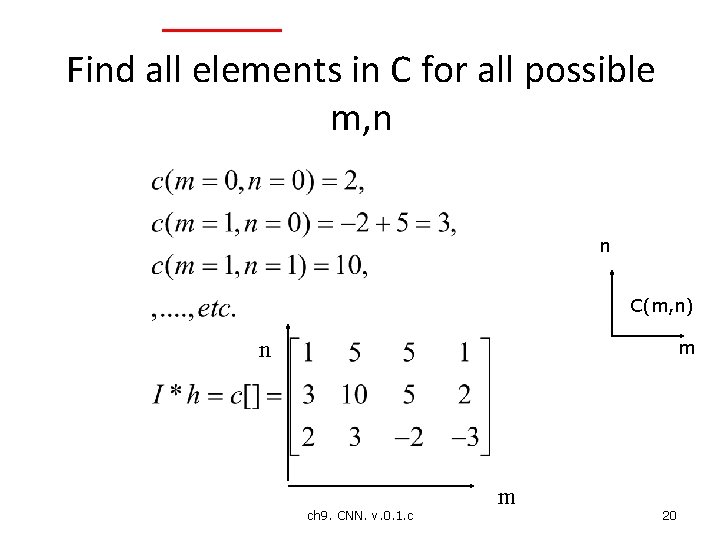
Find all elements in C for all possible m, n n C(m, n) n m ch 9. CNN. v. 0. 1. c m 20

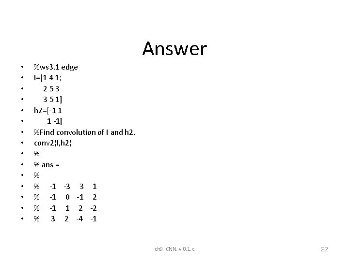
Exercise • • • I=[1 4 1; 2 5 3 3 5 1] h 2=[-1 1 1 -1] Find convolution of I and h 2. ch 9. CNN. v. 0. 1. c 21

Answer • • • • %ws 3. 1 edge I=[1 4 1; 2 5 3 3 5 1] h 2=[-1 1 1 -1] %Find convolution of I and h 2. conv 2(I, h 2) % % ans = % % -1 -3 3 1 % -1 0 -1 2 % -1 1 2 -2 % 3 2 -4 -1 ch 9. CNN. v. 0. 1. c 22

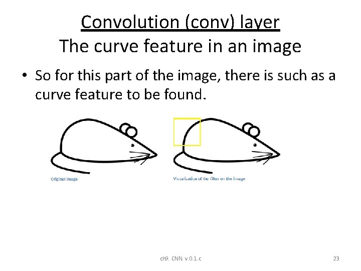
Convolution (conv) layer The curve feature in an image • So for this part of the image, there is such as a curve feature to be found. ch 9. CNN. v. 0. 1. c 23

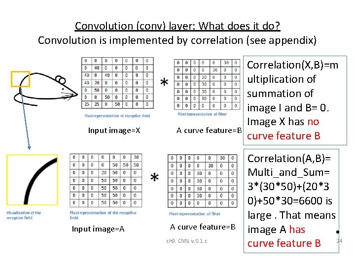
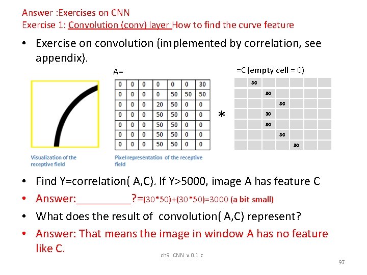
Convolution (conv) layer: What does it do? Convolution is implemented by correlation (see appendix) Input image=X Input image=A A curve feature=B ch 9. CNN. v. 0. 1. c Correlation(X, B)=m ultiplication of summation of image I and B= 0. Image X has no curve feature B Correlation(A, B)= Multi_and_Sum= 3*(30*50)+(20*3 0)+50*30=6600 is large. That means image A has • curve feature B 24

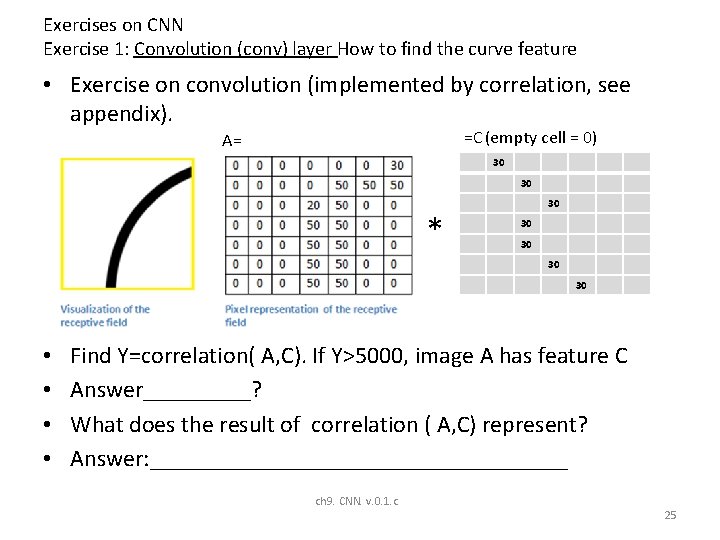
Exercises on CNN Exercise 1: Convolution (conv) layer How to find the curve feature • Exercise on convolution (implemented by correlation, see appendix). =C (empty cell = 0) A= 30 30 * 30 30 30 • • Find Y=correlation( A, C). If Y>5000, image A has feature C Answer_____? What does the result of correlation ( A, C) represent? Answer: __________________ ch 9. CNN. v. 0. 1. c 25

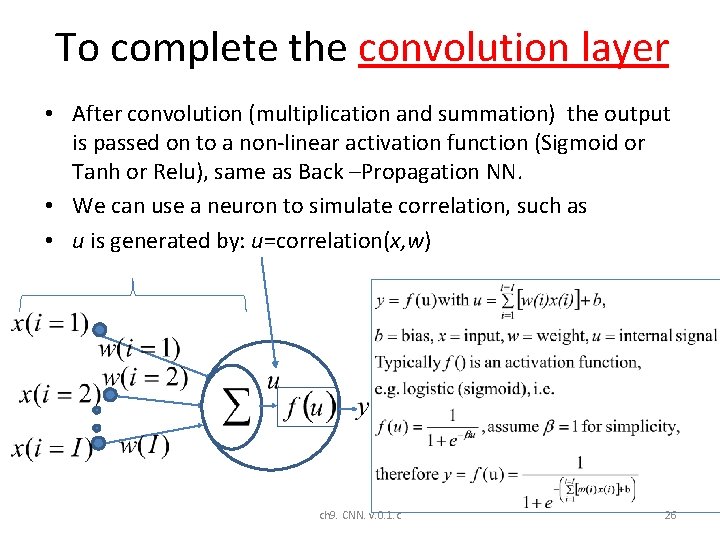
To complete the convolution layer • After convolution (multiplication and summation) the output is passed on to a non-linear activation function (Sigmoid or Tanh or Relu), same as Back –Propagation NN. • We can use a neuron to simulate correlation, such as • u is generated by: u=correlation(x, w) ch 9. CNN. v. 0. 1. c 26

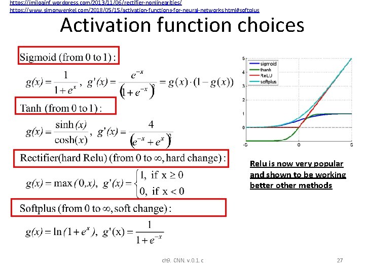
https: //imiloainf. wordpress. com/2013/11/06/rectifier-nonlinearities/ https: //www. simonwenkel. com/2018/05/15/activation-functions-for-neural-networks. html#softplus Activation function choices Relu is now very popular and shown to be working better other methods ch 9. CNN. v. 0. 1. c 27

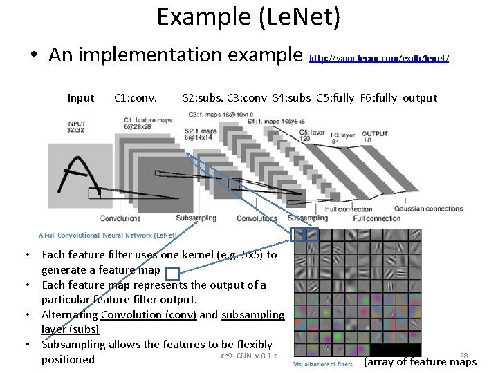
Example (Le. Net) • An implementation example http: //yann. lecun. com/exdb/lenet/ Input C 1: conv. S 2: subs. C 3: conv S 4: subs C 5: fully F 6: fully output • Each feature filter uses one kernel (e. g. 5 x 5) to generate a feature map • Each feature map represents the output of a particular feature filter output. • Alternating Convolution (conv) and subsampling layer (subs) • Subsampling allows the features to be flexibly ch 9. CNN. v. 0. 1. c positioned 28 (array of feature maps

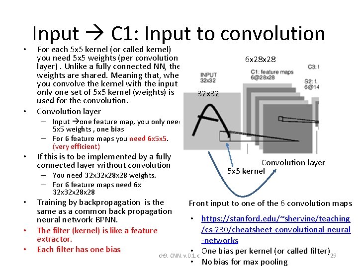
• • Input C 1: Input to convolution For each 5 x 5 kernel (or called kernel) you need 5 x 5 weights (per convolution layer). Unlike a fully connected NN, the weights are shared. Meaning that, when you convolve the kernel with the input , only one set of 5 x 5 kernel (weights) is used for the convolution. Convolution layer 6 x 28 32 x 32 – Input one feature map, you only need 5 x 5 weights , one bias – For 6 feature maps you need 6 x 5 x 5. (very efficient) • If this is to be implemented by a fully connected layer without convolution – You need 32 x 28 x 28 weights. – For 6 feature maps need 6 x 32 x 28 • • • Training by backpropagation is the same as a common back propagation neural network BPNN. The filter (kernel) is like a feature extractor. Each filter has one bias Convolution layer 5 x 5 kernel Front input to one of the 6 convolution maps • https: //stanford. edu/~shervine/teaching /cs-230/cheatsheet-convolutional-neural -networks • One bias per kernel (or called filter)29 ch 9. CNN. v. 0. 1. c • No bias for max pooling

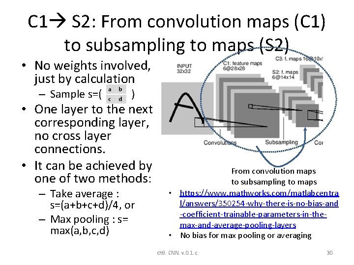
C 1 S 2: From convolution maps (C 1) to subsampling to maps (S 2) • No weights involved, just by calculation – Sample s=( ) • One layer to the next corresponding layer, no cross layer connections. • It can be achieved by one of two methods: – Take average : s=(a+b+c+d)/4, or – Max pooling : s= max(a, b, c, d) From convolution maps to subsampling to maps • https: //www. mathworks. com/matlabcentra l/answers/350254 -why-there-is-no-bias-and -coefficient-trainable-parameters-in-themax-and-average-pooling-layers • No bias for max pooling or averaging ch 9. CNN. v. 0. 1. c 30

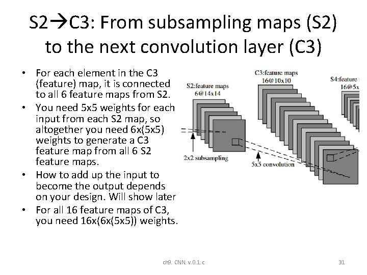
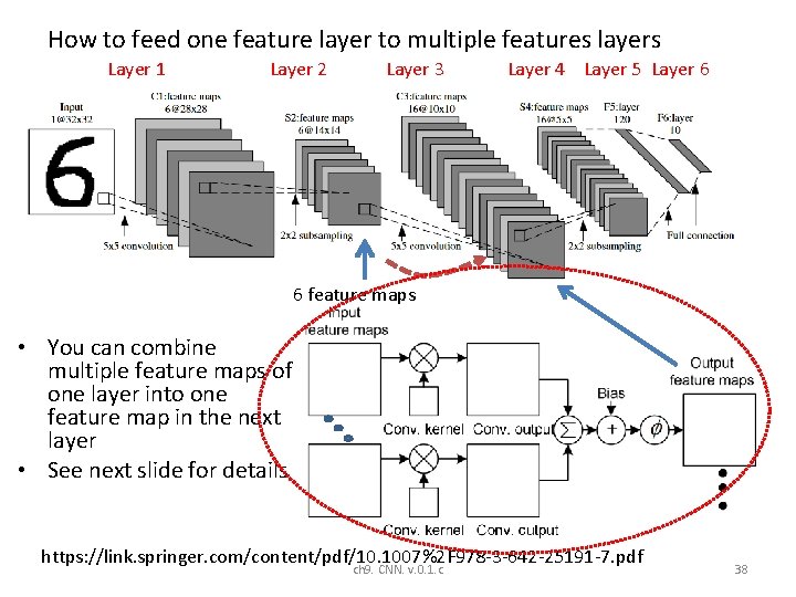
S 2 C 3: From subsampling maps (S 2) to the next convolution layer (C 3) • For each element in the C 3 (feature) map, it is connected to all 6 feature maps from S 2. • You need 5 x 5 weights for each input from each S 2 map, so altogether you need 6 x(5 x 5) weights to generate a C 3 feature map from all 6 S 2 feature maps. • How to add up the input to become the output depends on your design. Will show later • For all 16 feature maps of C 3, you need 16 x(6 x(5 x 5)) weights. ch 9. CNN. v. 0. 1. c 31

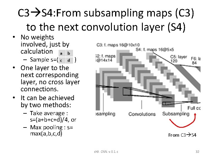
C 3 S 4: From subsampling maps (C 3) to the next convolution layer (S 4) • No weights involved, just by calculation – Sample s=( ) • One layer to the next corresponding layer, no cross layer connections. • It can be achieved by two methods: – Take average : s=(a+b+c+d)/4, or – Max pooling : s= max(a, b, c, d) From C 3 S 4 ch 9. CNN. v. 0. 1. c 32

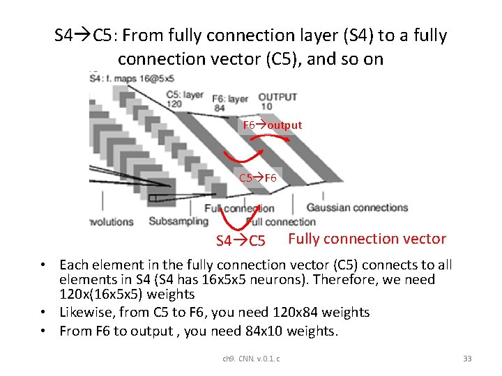
S 4 C 5: From fully connection layer (S 4) to a fully connection vector (C 5), and so on F 6 output C 5 F 6 S 4 C 5 Fully connection vector • Each element in the fully connection vector (C 5) connects to all elements in S 4 (S 4 has 16 x 5 x 5 neurons). Therefore, we need 120 x(16 x 5 x 5) weights • Likewise, from C 5 to F 6, you need 120 x 84 weights • From F 6 to output , you need 84 x 10 weights. ch 9. CNN. v. 0. 1. c 33

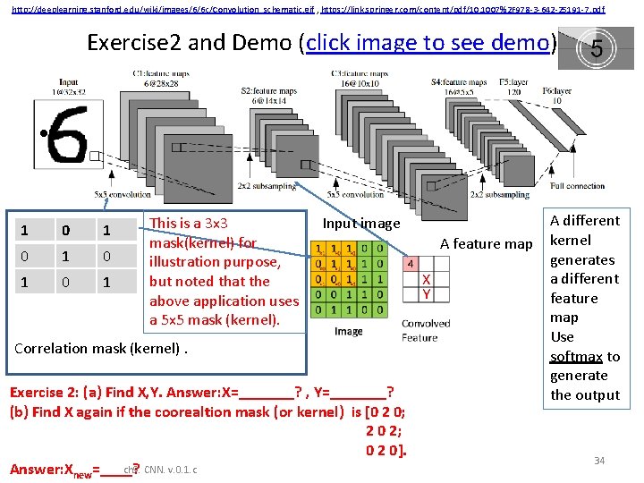
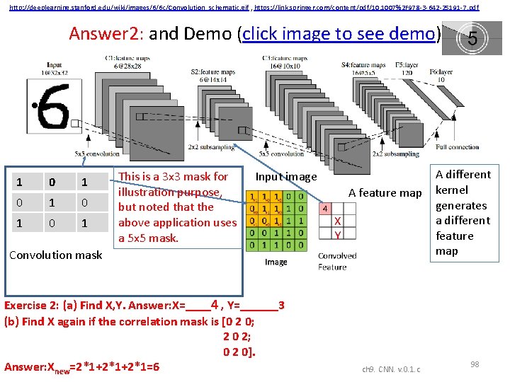
http: //deeplearning. stanford. edu/wiki/images/6/6 c/Convolution_schematic. gif , https: //link. springer. com/content/pdf/10. 1007%2 F 978 -3 -642 -25191 -7. pdf Exercise 2 and Demo (click image to see demo) • 1 0 1 0 1 This is a 3 x 3 mask(kernel) for illustration purpose, but noted that the above application uses a 5 x 5 mask (kernel). Input image A feature map X Y Correlation mask (kernel). Exercise 2: (a) Find X, Y. Answer: X=_______? , Y=_______? (b) Find X again if the coorealtion mask (or kernel) is [0 2 0; 2 0 2; 0 2 0]. ch 9. CNN. v. 0. 1. c Answer: Xnew=____? A different kernel generates a different feature map Use softmax to generate the output 34

Description of the layers Subsampling Layer to layer connections ch 9. CNN. v. 0. 1. c 35

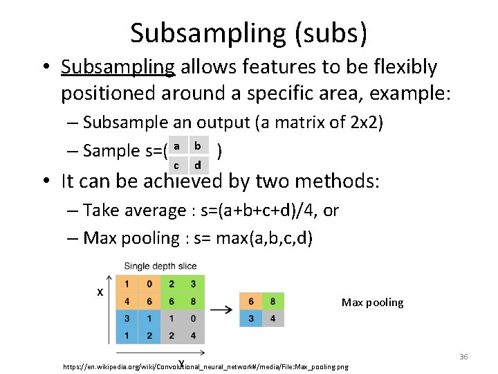
Subsampling (subs) • Subsampling allows features to be flexibly positioned around a specific area, example: – Subsample an output (a matrix of 2 x 2) a b – Sample s=( ) c d • It can be achieved by two methods: – Take average : s=(a+b+c+d)/4, or – Max pooling : s= max(a, b, c, d) Max pooling ch 9. CNN. v. 0. 1. c https: //en. wikipedia. org/wiki/Convolutional_neural_network#/media/File: Max_pooling. png 36

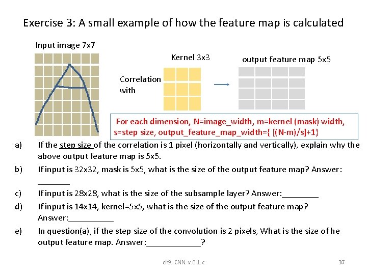
Exercise 3: A small example of how the feature map is calculated Input image 7 x 7 Kernel 3 x 3 output feature map 5 x 5 Correlation with a) b) c) d) e) For each dimension, N=image_width, m=kernel (mask) width, s=step size, output_feature_map_width={ [(N-m)/s]+1} If the step size of the correlation is 1 pixel (horizontally and vertically), explain why the above output feature map is 5 x 5. If input is 32 x 32, mask is 5 x 5, what is the size of the output feature map? Answer: _______ If input is 28 x 28, what is the size of the subsample layer? Answer: ____ If input is 14 x 14, kernel=5 x 5, what is the size of the output feature map? Answer: _____ In question(a), if the step size of the convolution is 2 pixels, What is the size of he output feature map. Answer: ______? 3 x 3 ch 9. CNN. v. 0. 1. c 37

How to feed one feature layer to multiple features layers Layer 1 Layer 2 Layer 3 Layer 4 Layer 5 Layer 6 6 feature maps • You can combine multiple feature maps of one layer into one feature map in the next layer • See next slide for details https: //link. springer. com/content/pdf/10. 1007%2 F 978 -3 -642 -25191 -7. pdf ch 9. CNN. v. 0. 1. c 38

• ch 9. CNN. v. 0. 1. c 39

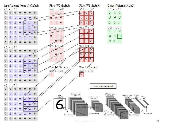
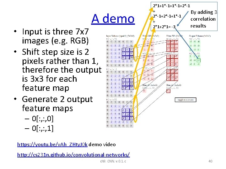
A demo • Input is three 7 x 7 images (e. g. RGB) • Shift step size is 2 pixels rather than 1, therefore the output is 3 x 3 for each feature map • Generate 2 output feature maps 2*1+1*-1+2*-1 + By adding 3 2*-1+1*-1 correlation + results 2*1+2*1= -3 – 0[: , 0] – 0[: , 1] https: //youtu. be/v. Ah_ZHty. J 0 k demo video http: //cs 231 n. github. io/convolutional-networks/ ch 9. CNN. v. 0. 1. c 40

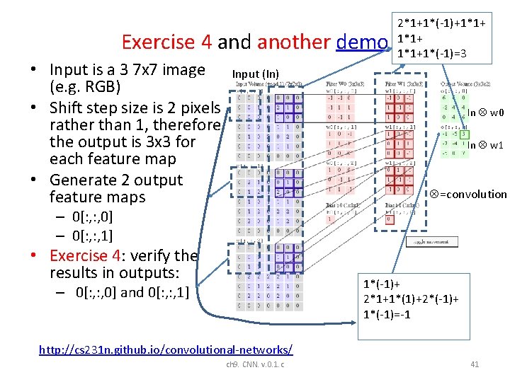
Exercise 4 and another demo • Input is a 3 7 x 7 image (e. g. RGB) • Shift step size is 2 pixels rather than 1, therefore the output is 3 x 3 for each feature map • Generate 2 output feature maps 2*1+1*(-1)+1*1+1*(-1)=3 Input (In) In w 0 In w 1 =convolution – 0[: , 0] – 0[: , 1] • Exercise 4: verify the results in outputs: 1*(-1)+ 2*1+1*(1)+2*(-1)+ 1*(-1)=-1 – 0[: , 0] and 0[: , 1] http: //cs 231 n. github. io/convolutional-networks/ ch 9. CNN. v. 0. 1. c 41

Example Using a program ch 9. CNN. v. 0. 1. c 42

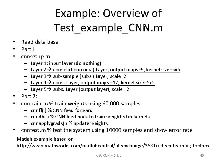
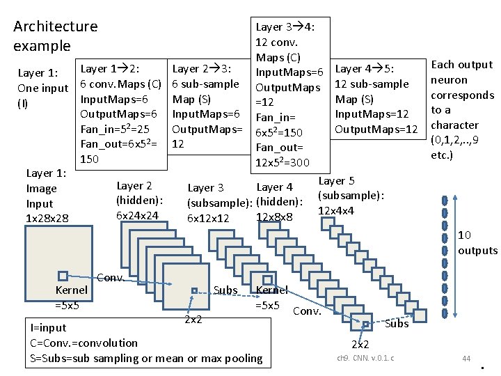
Example: Overview of Test_example_CNN. m • Read data base • Part I: • cnnsetup. m – – – Layer 1: input layer (do nothing) Layer 2 convolution(conv. ) Layer, output maps=6, kernel size=5 x 5 Layer 3 sub-sample (subs. ) Layer, scale=2 Layer 4 conv. Layer, output maps =12, kernel size=5 x 5 Layer 5 subs. Layer (output layer), scale =2 • Part 2: • cnntrain. m % train weights using 60, 000 samples – cnnff( ) % CNN feed forward – cnndb( ) % CNN feed back to train weighted in kernels – cnnapplygrads( ) % update weights • cnntest. m % test the system using 10000 samples and show error rate Matlab example based on http: //www. mathworks. com/matlabcentral/fileexchange/38310 -deep-learning-toolbox ch 9. CNN. v. 0. 1. c 43

Architecture example Layer 3 4: 12 conv. Maps (C) Layer 1 2: Layer 2 3: Input. Maps=6 Layer 4 5: Layer 1: One input 6 conv. Maps (C) 6 sub-sample Output. Maps 12 sub-sample Input. Maps=6 Map (S) =12 (I) Output. Maps=6 Input. Maps=6 Fan_in= Input. Maps=12 Fan_in=52=25 Output. Maps=12 Output. Maps= 6 x 52=150 Fan_out=6 x 52= 12 Fan_out= 150 12 x 52=300 Layer 1: Layer 5 Layer 2 Layer 4 Layer 3 Image (subsample): (hidden): Input 12 x 4 x 4 6 x 24 12 x 8 x 8 6 x 12 1 x 28 Each output neuron corresponds to a character (0, 1, 2, . . , 9 etc. ) 10 outputs Kernel =5 x 5 Conv. Subs Kernel =5 x 5 Conv. 2 x 2 I=input C=Conv. =convolution S=Subs=sub sampling or mean or max pooling Subs 2 x 2 ch 9. CNN. v. 0. 1. c 44 •

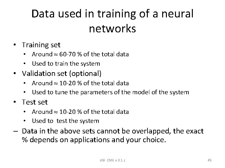
Data used in training of a neural networks • Training set • Around 60 -70 % of the total data • Used to train the system • Validation set (optional) • Around 10 -20 % of the total data • Used to tune the parameters of the model of the system • Test set • Around 10 -20 % of the total data • Used to test the system – Data in the above sets cannot be overlapped, the exact % depends on applications and your choice. ch 9. CNN. v. 0. 1. c 45

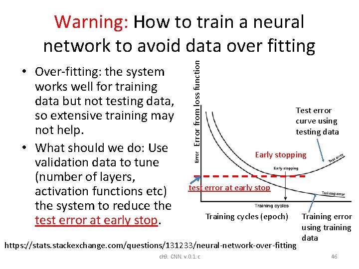
• Over-fitting: the system works well for training data but not testing data, so extensive training may not help. • What should we do: Use validation data to tune (number of layers, activation functions etc) the system to reduce the test error at early stop. Error from loss function Warning: How to train a neural network to avoid data over fitting Test error curve using testing data Early stopping test error at early stop Training cycles (epoch) https: //stats. stackexchange. com/questions/131233/neural-network-over-fitting ch 9. CNN. v. 0. 1. c Training error using training data 46

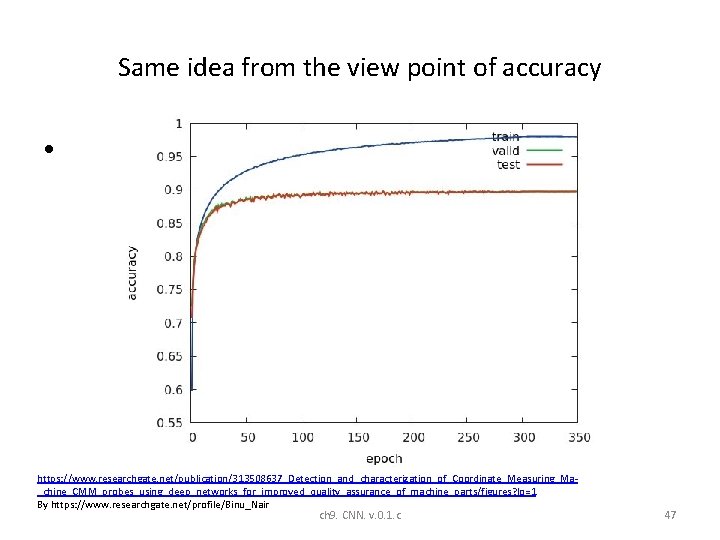
Same idea from the view point of accuracy • https: //www. researchgate. net/publication/313508637_Detection_and_characterization_of_Coordinate_Measuring_Ma_chine_CMM_probes_using_deep_networks_for_improved_quality_assurance_of_machine_parts/figures? lo=1 By https: //www. researchgate. net/profile/Binu_Nair ch 9. CNN. v. 0. 1. c 47

Part A. 2 Feedforward details Feed forward part of cnnff( ) Matlab example http: //www. mathworks. com/matlabcentral/fileexchange/38310 -deep-learning-toolbox ch 9. CNN. v. 0. 1. c 48

Cnnff. m Convolution Neural Networks feed forward • This is the feed forward part • Assume all the weights are initialized or calculated, we show to get the output from inputs. • Ref: CNN Matlab example http: //www. mathworks. com/matlabcentral/fileexch ange/38310 -deep-learning-toolbox ch 9. CNN. v. 0. 1. c 49

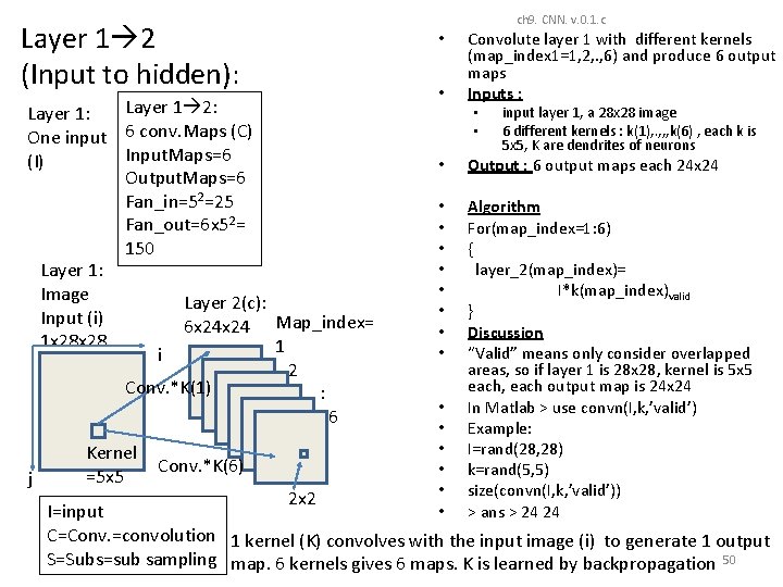
Layer 1 2 (Input to hidden): Layer 1 2: Layer 1: One input 6 conv. Maps (C) Input. Maps=6 (I) Output. Maps=6 Fan_in=52=25 Fan_out=6 x 52= 150 Layer 1: Image Layer 2(c): Input (i) 6 x 24 Map_index= 1 x 28 1 i 2 Conv. *K(1) : 6 j Kernel =5 x 5 Conv. *K(6) ch 9. CNN. v. 0. 1. c • • Convolute layer 1 with different kernels (map_index 1=1, 2, . , 6) and produce 6 output maps Inputs : • • input layer 1, a 28 x 28 image 6 different kernels : k(1), . , , , k(6) , each k is 5 x 5, K are dendrites of neurons • Output : 6 output maps each 24 x 24 • • Algorithm For(map_index=1: 6) { layer_2(map_index)= I*k(map_index)valid } Discussion “Valid” means only consider overlapped areas, so if layer 1 is 28 x 28, kernel is 5 x 5 each, each output map is 24 x 24 In Matlab > use convn(I, k, ’valid’) Example: I=rand(28, 28) k=rand(5, 5) size(convn(I, k, ’valid’)) > ans > 24 24 • • • 2 x 2 I=input C=Conv. =convolution 1 kernel (K) convolves with the input image (i) to generate 1 output S=Subs=sub sampling map. 6 kernels gives 6 maps. K is learned by backpropagation 50

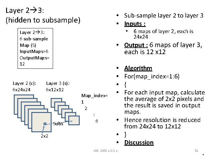
Layer 2 3: (hidden to subsample) • Sub-sample layer 2 to layer 3 • Inputs : • 6 maps of layer 2, each is 24 x 24 Layer 2 3: 6 sub-sample Map (S) Input. Maps=6 Output. Maps= 12 Layer 2 (c): 6 x 24 • Output : 6 maps of layer 3, each is 12 x 12 Layer 3 (s): 6 x 12 Subs 2 x 2 Map_index= 1 2 : 6 Algorithm For(map_index=1: 6) { For each input map, calculate the average of 2 x 2 pixels and the result is saved in output maps. • Hence resolution is reduced from 24 x 24 to 12 x 12 • } • Discussion • • ch 9. CNN. v. 0. 1. c 51 •

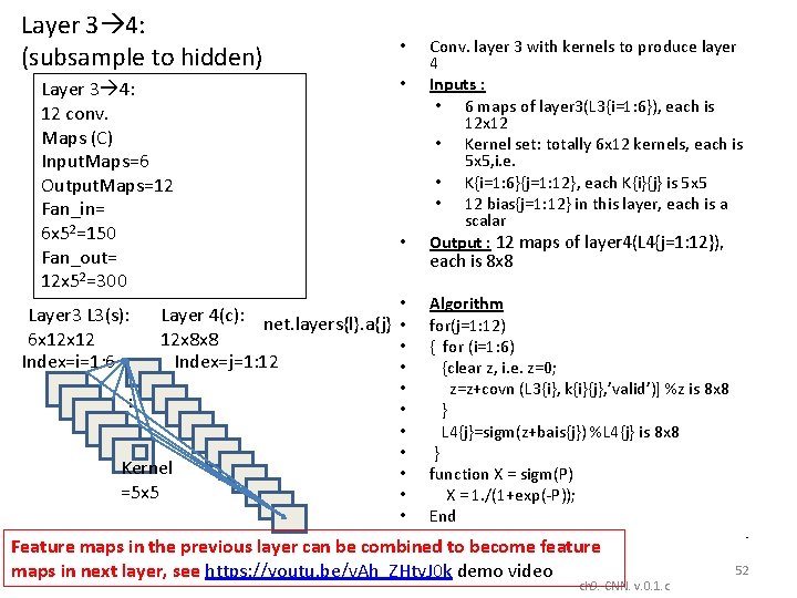
Layer 3 4: (subsample to hidden) Layer 3 4: 12 conv. Maps (C) Input. Maps=6 Output. Maps=12 Fan_in= 6 x 52=150 Fan_out= 12 x 52=300 Layer 3 L 3(s): 6 x 12 Index=i=1: 6 • • Layer 4(c): net. layers{l}. a{j} • 12 x 8 x 8 • Index=j=1: 12 • : Kernel =5 x 5 • • Conv. layer 3 with kernels to produce layer 4 Inputs : • 6 maps of layer 3(L 3{i=1: 6}), each is 12 x 12 • Kernel set: totally 6 x 12 kernels, each is 5 x 5, i. e. • K{i=1: 6}{j=1: 12}, each K{i}{j} is 5 x 5 • 12 bias{j=1: 12} in this layer, each is a scalar Output : 12 maps of layer 4(L 4{j=1: 12}), each is 8 x 8 Algorithm for(j=1: 12) { for (i=1: 6) {clear z, i. e. z=0; z=z+covn (L 3{i}, k{i}{j}, ’valid’)] %z is 8 x 8 } L 4{j}=sigm(z+bais{j}) %L 4{j} is 8 x 8 } function X = sigm(P) X = 1. /(1+exp(-P)); End Feature maps in the previous layer can be combined to become feature maps in next layer, see https: //youtu. be/v. Ah_ZHty. J 0 k demo video ch 9. CNN. v. 0. 1. c • 52

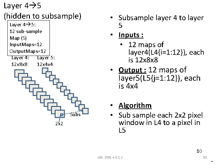
Layer 4 5 (hidden to subsample) Layer 4 5: 12 sub-sample Map (S) Input. Maps=12 Output. Maps=12 Layer 4: Layer 5: 12 x 8 x 8 12 x 4 x 4 • Subsample layer 4 to layer 5 • Inputs : • 12 maps of layer 4(L 4{i=1: 12}), each is 12 x 8 x 8 • Output : 12 maps of layer 5(L 5{j=1: 12}), each is 4 x 4 Subs 2 x 2 • Algorithm • Sub sample each 2 x 2 pixel window in L 4 to a pixel in L 5 10 ch 9. CNN. v. 0. 1. c 53 •

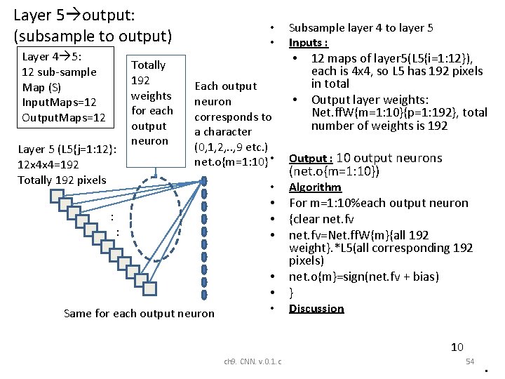
Layer 5 output: (subsample to output) Layer 4 5: 12 sub-sample Map (S) Input. Maps=12 Output. Maps=12 Layer 5 (L 5{j=1: 12}: 12 x 4 x 4=192 Totally 192 pixels Totally 192 weights for each output neuron • • Subsample layer 4 to layer 5 Inputs : • Each output neuron corresponds to a character (0, 1, 2, . . , 9 etc. ) net. o{m=1: 10} • : : • • • Same for each output neuron • • 12 maps of layer 5(L 5{i=1: 12}), each is 4 x 4, so L 5 has 192 pixels in total Output layer weights: Net. ff. W{m=1: 10}{p=1: 192}, total number of weights is 192 Output : 10 output neurons (net. o{m=1: 10}) Algorithm For m=1: 10%each output neuron {clear net. fv=Net. ff. W{m}{all 192 weight}. *L 5(all corresponding 192 pixels) net. o{m}=sign(net. fv + bias) } Discussion 10 ch 9. CNN. v. 0. 1. c 54 •

Part A. 3 Back propagation details Back propagation part cnnbp( ) cnnapplyweight( ) ch 9. CNN. v. 0. 1. c 55

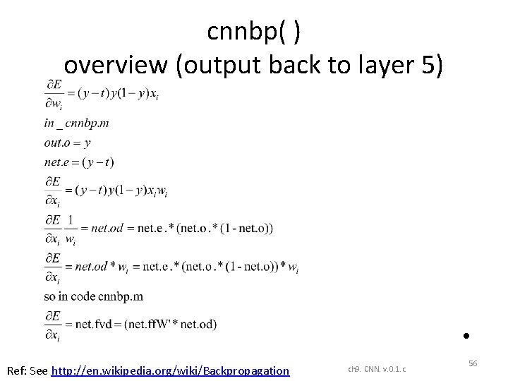
cnnbp( ) overview (output back to layer 5) • Ref: See http: //en. wikipedia. org/wiki/Backpropagation ch 9. CNN. v. 0. 1. c 56

Calculate gradient • • • From later 2 to layer 3 From later 3 to layer 4 Net. ff. W Net. ffb found The method is similar to a typical Back propagation neural network BPNN ch 9. CNN. v. 0. 1. c 57

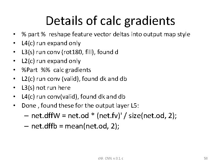
Details of calc gradients • • • % part % reshape feature vector deltas into output map style L 4(c) run expand only L 3(s) run conv (rot 180, fill), found d L 2(c) run expand only %Part %% calc gradients L 2(c) run conv (valid), found dk and db L 3(s) not run here L 4(c) run conv(valid), found dk and db Done , found these for the output layer L 5: – net. dff. W = net. od * (net. fv)' / size(net. od, 2); – net. dffb = mean(net. od, 2); ch 9. CNN. v. 0. 1. c 58

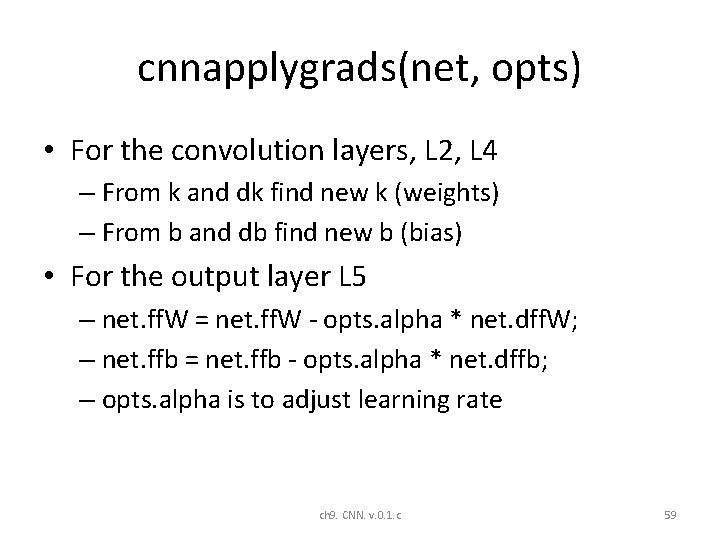
cnnapplygrads(net, opts) • For the convolution layers, L 2, L 4 – From k and dk find new k (weights) – From b and db find new b (bias) • For the output layer L 5 – net. ff. W = net. ff. W - opts. alpha * net. dff. W; – net. ffb = net. ffb - opts. alpha * net. dffb; – opts. alpha is to adjust learning rate ch 9. CNN. v. 0. 1. c 59

Part B: CNN Architectures History and descriptions ch 9. CNN. v. 0. 1. c 60

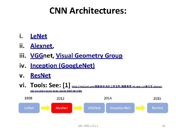
CNN Architectures: i. iii. iv. v. vi. Le. Net Alexnet, VGGnet, Visual Geometry Group Inception (Goog. Le. Net) Res. Net Tools: See: [1] https: //medium. com/雞雞與兔兔的 程世界/機器學習-ml-note-cnn演化史-alexnet- vgg-inception-resnet-keras-coding-668 f 74879306 ch 9. CNN. v. 0. 1. c 61

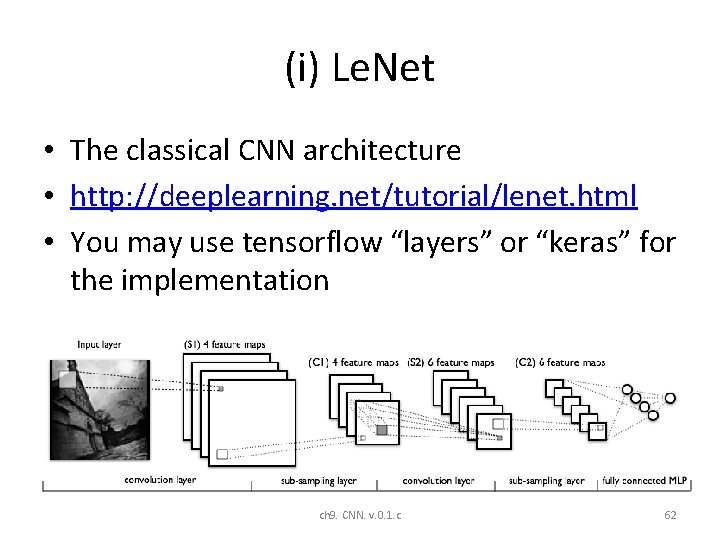
(i) Le. Net • The classical CNN architecture • http: //deeplearning. net/tutorial/lenet. html • You may use tensorflow “layers” or “keras” for the implementation ch 9. CNN. v. 0. 1. c 62

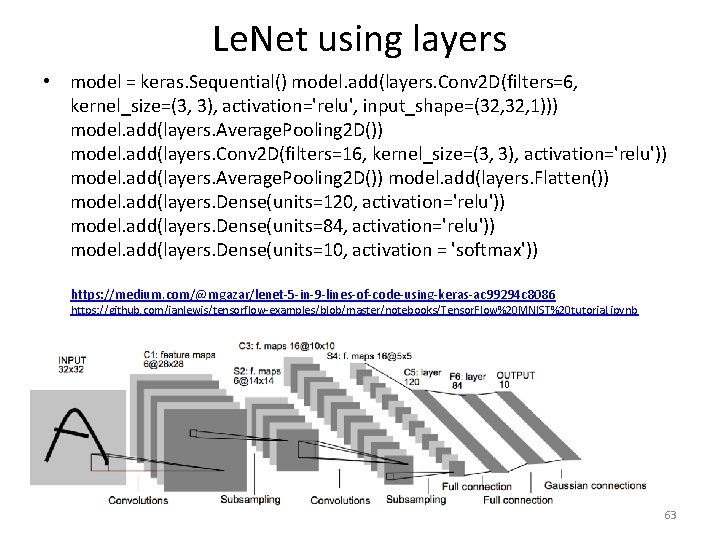
Le. Net using layers • model = keras. Sequential() model. add(layers. Conv 2 D(filters=6, kernel_size=(3, 3), activation='relu', input_shape=(32, 1))) model. add(layers. Average. Pooling 2 D()) model. add(layers. Conv 2 D(filters=16, kernel_size=(3, 3), activation='relu')) model. add(layers. Average. Pooling 2 D()) model. add(layers. Flatten()) model. add(layers. Dense(units=120, activation='relu')) model. add(layers. Dense(units=84, activation='relu')) model. add(layers. Dense(units=10, activation = 'softmax')) https: //medium. com/@mgazar/lenet-5 -in-9 -lines-of-code-using-keras-ac 99294 c 8086 https: //github. com/ianlewis/tensorflow-examples/blob/master/notebooks/Tensor. Flow%20 MNIST%20 tutorial. ipynb ch 9. CNN. v. 0. 1. c 63

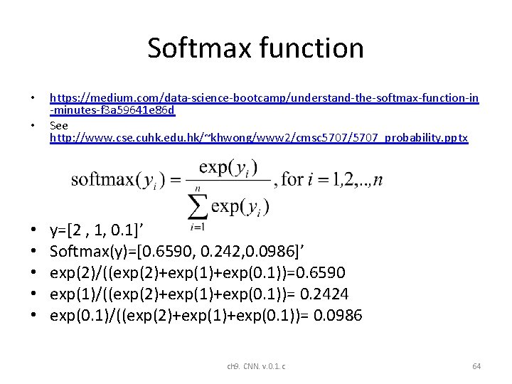
Softmax function • • https: //medium. com/data-science-bootcamp/understand-the-softmax-function-in -minutes-f 3 a 59641 e 86 d See http: //www. cse. cuhk. edu. hk/~khwong/www 2/cmsc 5707/5707_probability. pptx y=[2 , 1, 0. 1]’ Softmax(y)=[0. 6590, 0. 242, 0. 0986]’ exp(2)/((exp(2)+exp(1)+exp(0. 1))=0. 6590 exp(1)/((exp(2)+exp(1)+exp(0. 1))= 0. 2424 exp(0. 1)/((exp(2)+exp(1)+exp(0. 1))= 0. 0986 ch 9. CNN. v. 0. 1. c 64

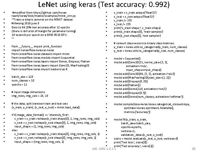
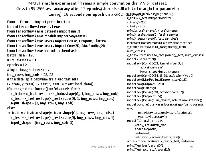
Le. Net using keras (Test accuracy: 0. 992) • • • #modified from https: //github. com/kerasteam/keras/blob/master/examples/mnist_cnn. py '''Trains a simple convnet on the MNIST dataset. #khwong 2019 june 8 Gets to 99. 25% test accuracy after 12 epochs (there is still a lot of margin for parameter tuning). 16 seconds per epoch on a GRID K 520 GPU. ''' • • from __future__ import print_function import tensorflow. keras as keras from tensorflow. keras. datasets import mnist from tensorflow. keras. models import Sequential from tensorflow. keras. layers import Dense, Dropout, Flatten from tensorflow. keras. layers import Conv 2 D, Max. Pooling 2 D from tensorflow. keras import backend as K • • • batch_size = 128 num_classes = 10 epochs = 12 • • # input image dimensions img_rows, img_cols = 28, 28 • • # the data, split between train and test sets (x_train, y_train), (x_test, y_test) = mnist. load_data() • • if K. image_data_format() == 'channels_first': x_train = x_train. reshape(x_train. shape[0], 1, img_rows, img_cols) x_test = x_test. reshape(x_test. shape[0], 1, img_rows, img_cols) input_shape = (1, img_rows, img_cols) else: x_train = x_train. reshape(x_train. shape[0], img_rows, img_cols, 1) x_test = x_test. reshape(x_test. shape[0], img_rows, img_cols, 1) input_shape = (img_rows, img_cols, 1) • • x_train = x_train. astype('float 32') x_test = x_test. astype('float 32') x_train /= 255 x_test /= 255 print('x_train shape: ', x_train. shape) print(x_train. shape[0], 'train samples') print(x_test. shape[0], 'test samples') • • • # convert class vectors to binary class matrices y_train = keras. utils. to_categorical(y_train, num_classes) y_test = keras. utils. to_categorical(y_test, num_classes) • • • model = Sequential() model. add(Conv 2 D(32, kernel_size=(3, 3), activation='relu', input_shape=input_shape)) model. add(Conv 2 D(64, (3, 3), activation='relu')) model. add(Max. Pooling 2 D(pool_size=(2, 2))) model. add(Dropout(0. 25)) model. add(Flatten()) model. add(Dense(128, activation='relu')) model. add(Dropout(0. 5)) model. add(Dense(num_classes, activation='softmax')) • • • model. compile(loss=keras. losses. categorical_crossentropy, optimizer=keras. optimizers. Adadelta(), metrics=['accuracy']) • model. fit(x_train, y_train, • batch_size=batch_size, • epochs=epochs, • verbose=1, • validation_data=(x_test, y_test)) • score = model. evaluate(x_test, y_test, verbose=0) • print('Test loss: ', score[0]) • print('Test accuracy: ', score[1]) ch 9. CNN. v. 0. 1. c 65

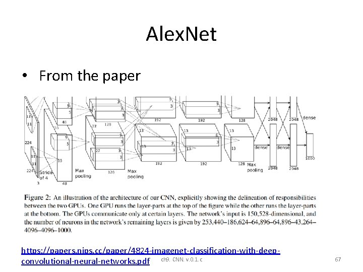
(ii) Alex. Net • https: //engmrk. com/alexnet-implementation-using-keras/ • https: //www. learnopencv. com/understanding-alexnet/ • Alex. Net – – – consists of 5 Convolutional Layers and 3 Fully Connected Layers Overlapping Max Pooling Re. LU Nonlinearity Reducing Overfitting Data Augmentation Dropout • Paper : https: //papers. nips. cc/paper/4824 -imagenetclassification-with-deep-convolutional-neural-networks. pdf ch 9. CNN. v. 0. 1. c 66

Alex. Net • From the paper https: //papers. nips. cc/paper/4824 -imagenet-classification-with-deepconvolutional-neural-networks. pdf ch 9. CNN. v. 0. 1. c 67

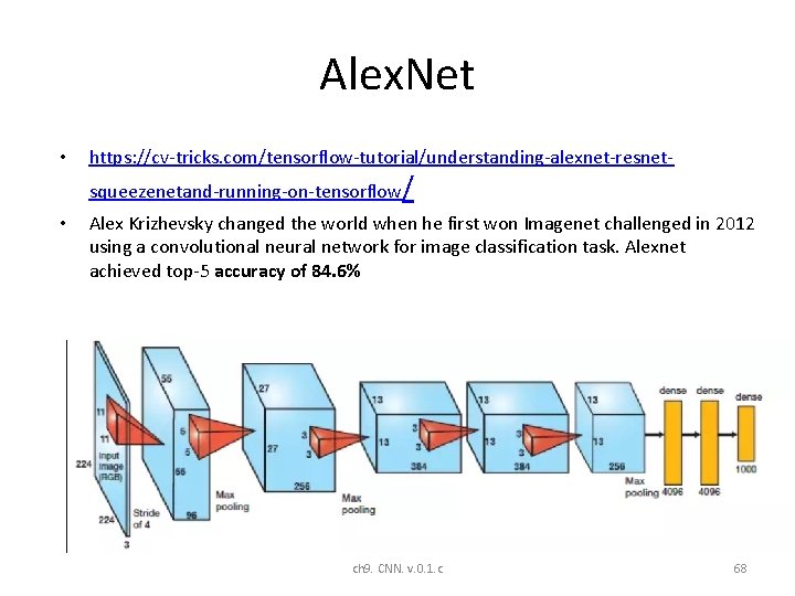
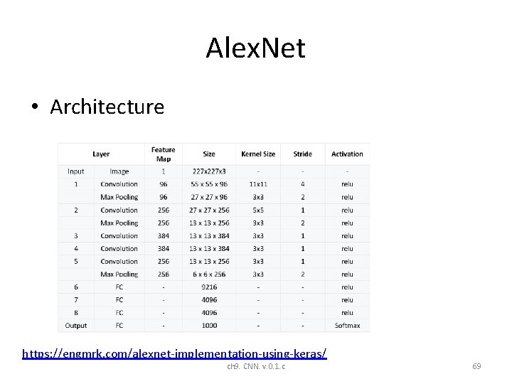
Alex. Net • https: //cv-tricks. com/tensorflow-tutorial/understanding-alexnet-resnetsqueezenetand-running-on-tensorflow/ • Alex Krizhevsky changed the world when he first won Imagenet challenged in 2012 using a convolutional neural network for image classification task. Alexnet achieved top-5 accuracy of 84. 6% ch 9. CNN. v. 0. 1. c 68

Alex. Net • Architecture https: //engmrk. com/alexnet-implementation-using-keras/ ch 9. CNN. v. 0. 1. c 69

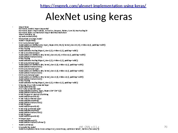
https: //engmrk. com/alexnet-implementation-using-keras/ Alex. Net using keras • • • • import keras from keras. models import Sequential from keras. layers import Dense, Activation, Dropout, Flatten, Conv 2 D, Max. Pooling 2 D from keras. layers. normalization import Batch. Normalization import numpy as np np. random. seed(1000) #Instantiate an empty model = Sequential() # 1 st Convolutional Layer model. add(Conv 2 D(filters=96, input_shape=(224, 3), kernel_size=(11, 11), strides=(4, 4), padding=’valid’)) model. add(Activation(‘relu’)) # Max Pooling model. add(Max. Pooling 2 D(pool_size=(2, 2), strides=(2, 2), padding=’valid’)) # 2 nd Convolutional Layer model. add(Conv 2 D(filters=256, kernel_size=(11, 11), strides=(1, 1), padding=’valid’)) model. add(Activation(‘relu’)) # Max Pooling model. add(Max. Pooling 2 D(pool_size=(2, 2), strides=(2, 2), padding=’valid’)) # 3 rd Convolutional Layer model. add(Conv 2 D(filters=384, kernel_size=(3, 3), strides=(1, 1), padding=’valid’)) model. add(Activation(‘relu’)) # 4 th Convolutional Layer model. add(Conv 2 D(filters=384, kernel_size=(3, 3), strides=(1, 1), padding=’valid’)) model. add(Activation(‘relu’)) # 5 th Convolutional Layer model. add(Conv 2 D(filters=256, kernel_size=(3, 3), strides=(1, 1), padding=’valid’)) model. add(Activation(‘relu’)) # Max Pooling model. add(Max. Pooling 2 D(pool_size=(2, 2), strides=(2, 2), padding=’valid’)) # Passing it to a Fully Connected layer model. add(Flatten()) # 1 st Fully Connected Layer model. add(Dense(4096, input_shape=(224*3, ))) model. add(Activation(‘relu’)) # Add Dropout to prevent overfitting model. add(Dropout(0. 4)) # 2 nd Fully Connected Layer model. add(Dense(4096)) model. add(Activation(‘relu’)) # Add Dropout model. add(Dropout(0. 4)) # 3 rd Fully Connected Layer model. add(Dense(1000)) model. add(Activation(‘relu’)) # Add Dropout model. add(Dropout(0. 4)) # Output Layer model. add(Dense(17)) model. add(Activation(‘softmax’)) model. summary() # Compile the model ch 9. CNN. v. 0. 1. c model. compile(loss=keras. losses. categorical_crossentropy, optimizer=’adam’, metrics=[“accuracy”]) 70

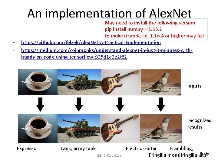
An implementation of Alex. Net • • May need to install the following version pip install numpy==1. 16. 2 to make it work, i. e. 1. 16. 4 or higher may fail https: //github. com/felzek/Alex. Net-A-Practical-Implementation https: //medium. com/coinmonks/understand-alexnet-in-just-3 -minutes-withhands-on-code-using-tensorflow-925 d 1 e 2 e 2 f 82 inputs recognized results Expresso Tank, army tank ch 9. CNN. v. 0. 1. c Electric Guitar Brambling, 71 Fringilla montifringilla 燕雀

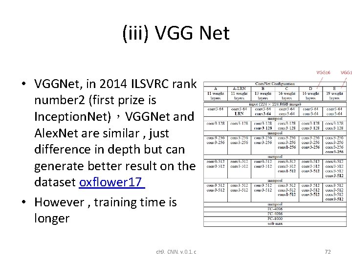
(iii) VGG Net • VGGNet, in 2014 ILSVRC rank number 2 (first prize is Inception. Net)，VGGNet and Alex. Net are similar , just difference in depth but can generate better result on the dataset oxflower 17 • However , training time is longer ch 9. CNN. v. 0. 1. c 72

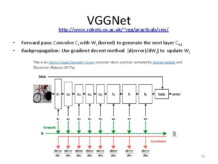
VGGNet http: //www. robots. ox. ac. uk/~vgg/practicals/cnn/ • • Forward pass: Convolve Ci with Wi (kernel) to generate the next layer Ci+1 Backpropagation: Use gradient decent method [d(error)/d. Wi] to update Wi ch 9. CNN. v. 0. 1. c 73

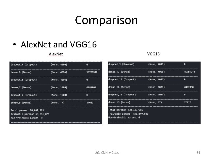
Comparison • Alex. Net and VGG 16 ch 9. CNN. v. 0. 1. c 74

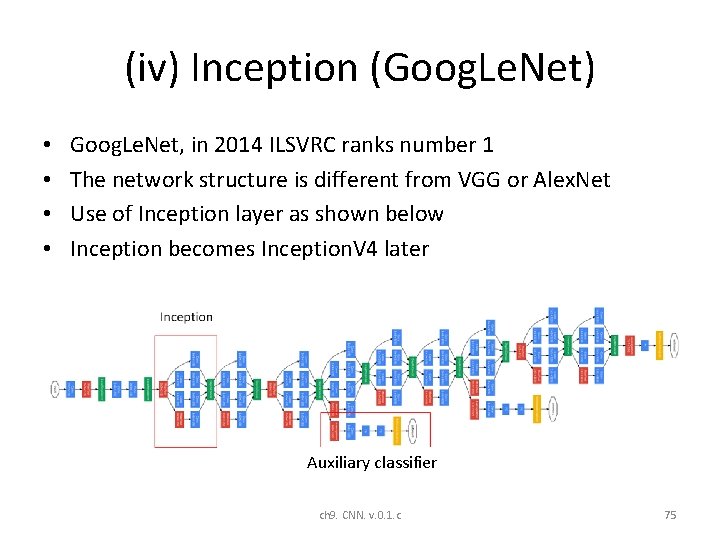
(iv) Inception (Goog. Le. Net) • • Goog. Le. Net, in 2014 ILSVRC ranks number 1 The network structure is different from VGG or Alex. Net Use of Inception layer as shown below Inception becomes Inception. V 4 later Auxiliary classifier ch 9. CNN. v. 0. 1. c 75

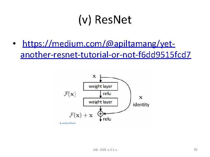
(v) Res. Net • https: //medium. com/@apiltamang/yetanother-resnet-tutorial-or-not-f 6 dd 9515 fcd 7 ch 9. CNN. v. 0. 1. c 76

(vi) Tools • Tensorflow , the current version includes Keras: The Python Deep Learning library • Microsoft CNTK • Caffé • Theano • Amazon Machine Learning • Torch • Brainstorm • http: //www. it 4 nextgen. com/best-artificialintelligence-frameworks/ ch 9. CNN. v. 0. 1. c 77

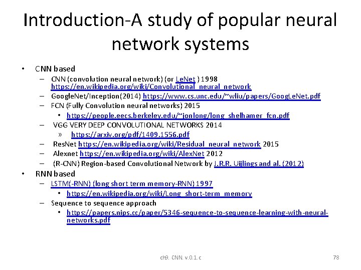
Introduction-A study of popular neural network systems • CNN based – CNN (convolution neural network) (or Le. Net ) 1998 https: //en. wikipedia. org/wiki/Convolutional_neural_network – Google. Net/Inception(2014) https: //www. cs. unc. edu/~wliu/papers/Goog. Le. Net. pdf – FCN (Fully Convolution neural networks) 2015 • https: //people. eecs. berkeley. edu/~jonlong/long_shelhamer_fcn. pdf – VGG VERY DEEP CONVOLUTIONAL NETWORKS 2014 » https: //arxiv. org/pdf/1409. 1556. pdf – Res. Net https: //en. wikipedia. org/wiki/Residual_neural_network 2015 – Alexnet https: //en. wikipedia. org/wiki/Alex. Net 2012 – (R-CNN) Region-based Convolutional Network by J. R. R. Uijlings and al. (2012) • RNN based – LSTM(-RNN) (long short term memory-RNN) 1997 • https: //en. wikipedia. org/wiki/Long_short-term_memory – Sequence to sequence approach • https: //papers. nips. cc/paper/5346 -sequence-to-sequence-learning-with-neuralnetworks. pdf ch 9. CNN. v. 0. 1. c 78

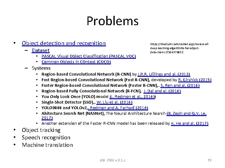
Problems • Object detection and recognition – Dataset • PASCAL Visual Object Classification (PASCAL VOC) • Common Objects in COntext (COCO) https: //medium. com/comet-app/review-ofdeep-learning-algorithms-for-objectdetection-c 1 f 3 d 437 b 852 – Systems Region-based Convolutional Network (R-CNN) by J. R. R. Uijlings and al. (2012) Fast Region-based Convolutional Network (Fast R-CNN), developed by R. Girshick (2015) Faster Region-based Convolutional Network (Faster R-CNN), . S. Ren and al. (2016) Region-based Fully Convolutional Network (R-FCN), J. Dai and al. (2016) You Only Look Once (YOLO) model (J. Redmon et al. , 2016)) Single-Shot Detector (SSD), , W. Liu et al. (2016) YOLO 9000 and YOLOv 2, . Redmon and A. Farhadi (2016) Ahitecture Search Net (NASNet), The Neural Architecture Search (B. Zoph and Q. V. Le, 2017) • Another extension of the Faster R-CNN model has been released by K. He and al. (2017) • • • Object tracking • Speech recognition • Machine translation ch 9. CNN. v. 0. 1. c 79

Summary • Studied the basic operation of Convolutional Neural networks (CNN) • Demonstrate how a simple CNN can be implemented ch 9. CNN. v. 0. 1. c 80

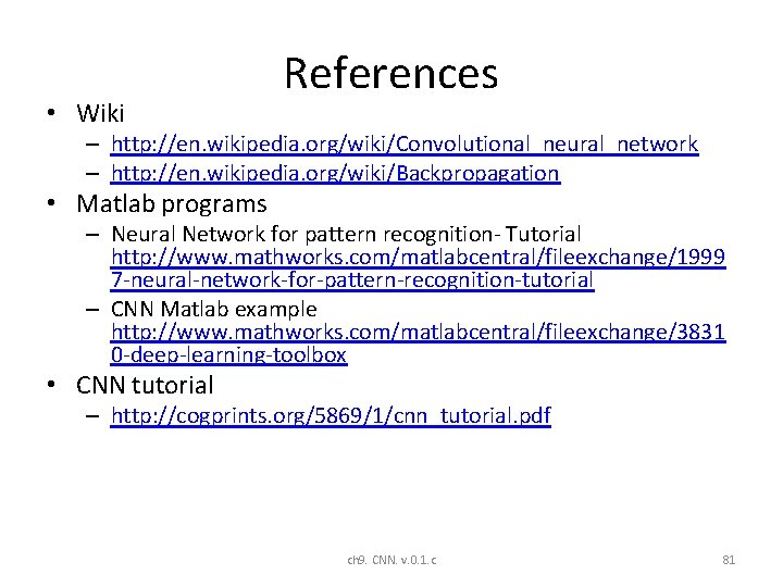
• Wiki References – http: //en. wikipedia. org/wiki/Convolutional_neural_network – http: //en. wikipedia. org/wiki/Backpropagation • Matlab programs – Neural Network for pattern recognition- Tutorial http: //www. mathworks. com/matlabcentral/fileexchange/1999 7 -neural-network-for-pattern-recognition-tutorial – CNN Matlab example http: //www. mathworks. com/matlabcentral/fileexchange/3831 0 -deep-learning-toolbox • CNN tutorial – http: //cogprints. org/5869/1/cnn_tutorial. pdf ch 9. CNN. v. 0. 1. c 81

Appendix ch 9. CNN. v. 0. 1. c 82

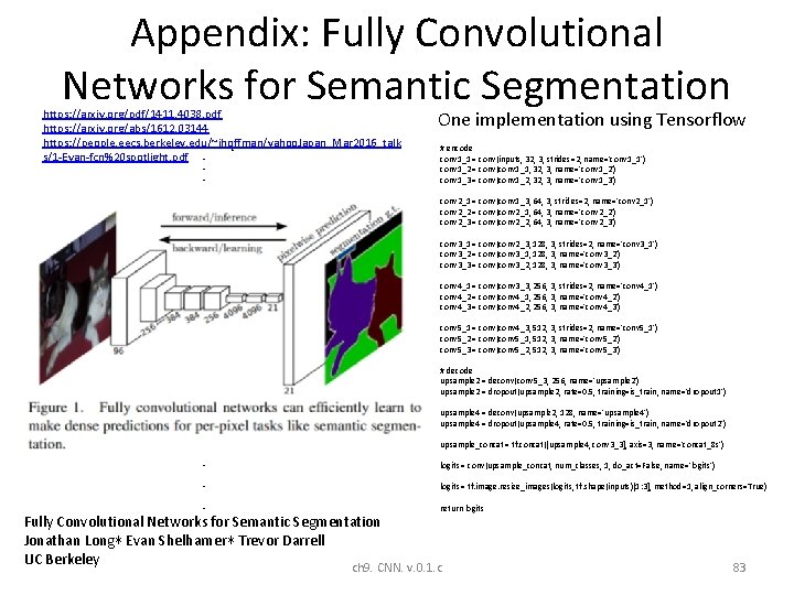
Appendix: Fully Convolutional Networks for Semantic Segmentation https: //arxiv. org/pdf/1411. 4038. pdf https: //arxiv. org/abs/1612. 03144 https: //people. eecs. berkeley. edu/~jhoffman/yahoo. Japan_Mar 2016_talk • c s/1 -Evan-fcn%20 spotlight. pdf • One implementation using Tensorflow • • # encode conv 1_1 = conv(inputs, 32, 3, strides=2, name='conv 1_1') conv 1_2 = conv(conv 1_1, 32, 3, name='conv 1_2') conv 1_3 = conv(conv 1_2, 3, name='conv 1_3') • • • conv 2_1 = conv(conv 1_3, 64, 3, strides=2, name='conv 2_1') conv 2_2 = conv(conv 2_1, 64, 3, name='conv 2_2') conv 2_3 = conv(conv 2_2, 64, 3, name='conv 2_3') • • • conv 3_1 = conv(conv 2_3, 128, 3, strides=2, name='conv 3_1') conv 3_2 = conv(conv 3_1, 128, 3, name='conv 3_2') conv 3_3 = conv(conv 3_2, 128, 3, name='conv 3_3') • • • conv 4_1 = conv(conv 3_3, 256, 3, strides=2, name='conv 4_1') conv 4_2 = conv(conv 4_1, 256, 3, name='conv 4_2') conv 4_3 = conv(conv 4_2, 256, 3, name='conv 4_3') • • • conv 5_1 = conv(conv 4_3, 512, 3, strides=2, name='conv 5_1') conv 5_2 = conv(conv 5_1, 512, 3, name='conv 5_2') conv 5_3 = conv(conv 5_2, 512, 3, name='conv 5_3') • • • # decode upsample 2 = deconv(conv 5_3, 256, name='upsample 2') upsample 2 = dropout(upsample 2, rate=0. 5, training=is_train, name='dropout 1') • • upsample 4 = deconv(upsample 2, 128, name='upsample 4') upsample 4 = dropout(upsample 4, rate=0. 5, training=is_train, name='dropout 2') • upsample_concat = tf. concat([upsample 4, conv 3_3], axis=3, name='concat_8 s') • logits = conv(upsample_concat, num_classes, 1, do_act=False, name='logits') • logits = tf. image. resize_images(logits, tf. shape(inputs)[1: 3], method=1, align_corners=True) • return logits Fully Convolutional Networks for Semantic Segmentation Jonathan Long∗ Evan Shelhamer∗ Trevor Darrell UC Berkeley ch 9. CNN. v. 0. 1. c 83

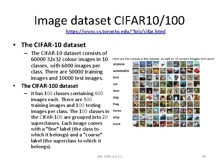
Image dataset CIFAR 10/100 https: //www. cs. toronto. edu/~kriz/cifar. html • The CIFAR-10 dataset • – The CIFAR-10 dataset consists of 60000 32 x 32 colour images in 10 classes, with 6000 images per class. There are 50000 training images and 10000 test images. The CIFAR-100 dataset – it has 100 classes containing 600 images each. There are 500 training images and 100 testing images per class. The 100 classes in the CIFAR-100 are grouped into 20 superclasses. Each image comes with a "fine" label (the class to which it belongs) and a "coarse" label (the superclass to which it belongs). ch 9. CNN. v. 0. 1. c 84

Tensor-flow experiments KH Wong ch 9. CNN. v. 0. 1. c 85

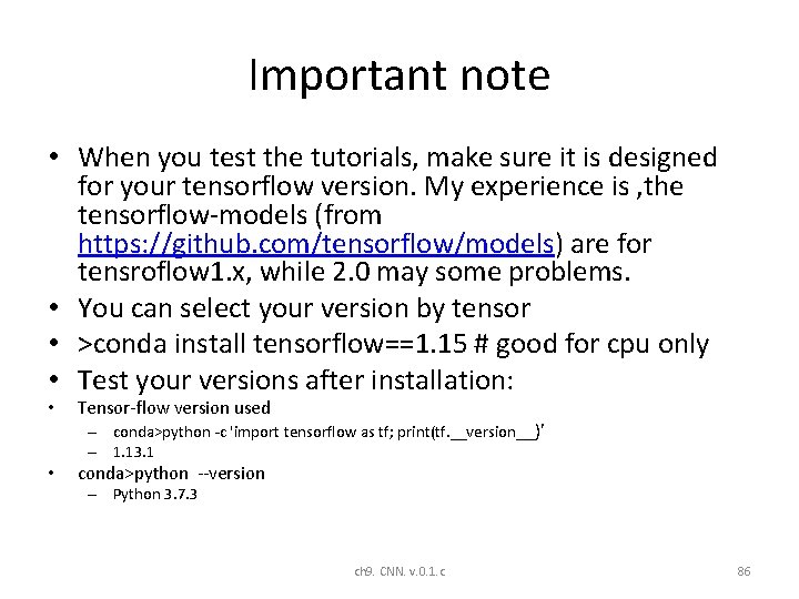
Important note • When you test the tutorials, make sure it is designed for your tensorflow version. My experience is , the tensorflow-models (from https: //github. com/tensorflow/models) are for tensroflow 1. x, while 2. 0 may some problems. • You can select your version by tensor • >conda install tensorflow==1. 15 # good for cpu only • Test your versions after installation: • Tensor-flow version used – conda>python -c 'import tensorflow as tf; print(tf. __version__)' – 1. 13. 1 • conda>python --version – Python 3. 7. 3 ch 9. CNN. v. 0. 1. c 86

Overview of Tensorflow • Installation • Tutorials: https: //www. tensorflow. org/tutorials – Tf-test 1: mnist, Optical Character recognition OCR – Tf-test 2: imagenet, , object recognition demo – Tf-test 2: alexnet, CNN, 1000 -object recognition – Tf-test 3: cifar 10, object recognition of 10 classes • https: //www. tensorflow. org/tutorials/images /transfer_learning ch 9. CNN. v. 0. 1. c 87

Useful links • Installation: https: //www. tensorflow. org/install • Tutorial: https: //www. tensorflow. org/tutorials • See tutorials of Github: https: //github. com/tensorflow/models – Tensorflowmodelstutorialsimage – alexnet – cifar 10_estimator – imagenet – mnist ch 9. CNN. v. 0. 1. c 88

Specific installation for We use win 10, anaconda • Installation instructions: • https: //sites. google. com/site/hongslinks/tens or_windows ch 9. CNN. v. 0. 1. c 89

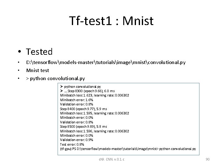
Tf-test 1 : Mnist • Tested • • • D: tensorflowmodels-mastertutorialsimagemnistconvolutional. py Mnist test > python convolutional. py Ø …. Step 8300 (epoch 9. 66), 6. 0 ms Minibatch loss: 1. 623, learning rate: 0. 006302 Minibatch error: 1. 6% Validation error: 0. 8% Step 8400 (epoch 9. 77), 5. 9 ms Minibatch loss: 1. 595, learning rate: 0. 006302 Minibatch error: 0. 0% Validation error: 0. 8% Step 8500 (epoch 9. 89), 5. 8 ms Minibatch loss: 1. 596, learning rate: 0. 006302 Minibatch error: 0. 0% Validation error: 0. 9% Test error: 0. 8% (tf-gpu) PS D: tensorflowmodels-mastertutorialsimagemnist> python convolutional. py ch 9. CNN. v. 0. 1. c 90

MNIST simple experiment: '''Trains a simple convnet on the MNIST dataset. Gets to 99. 25% test accuracy after 12 epochs, (there is still a lot of margin for parameter x_train = x_train. astype('float 32') tuning). 16 seconds per epoch on a GRID K 520 GPU. ''' from __future__ import print_function import tensorflow. keras as keras from tensorflow. keras. datasets import mnist from tensorflow. keras. models import Sequential from tensorflow. keras. layers import Dense, Dropout, Flatten from tensorflow. keras. layers import Conv 2 D, Max. Pooling 2 D from tensorflow. keras import backend as K batch_size = 128 num_classes = 10 epochs = 12 # input image dimensions img_rows, img_cols = 28, 28 # the data, split between train and test sets (x_train, y_train), (x_test, y_test) = mnist. load_data() if K. image_data_format() == 'channels_first': x_train = x_train. reshape(x_train. shape[0], 1, img_rows, img_cols) x_test = x_test. reshape(x_test. shape[0], 1, img_rows, img_cols) input_shape = (1, img_rows, img_cols) else: x_train = x_train. reshape(x_train. shape[0], img_rows, img_cols, 1) x_test = x_test. reshape(x_test. shape[0], img_rows, img_cols, 1) input_shape = (img_rows, img_cols, 1) ch 9. CNN. v. 0. 1. c x_test = x_test. astype('float 32') x_train /= 255 x_test /= 255 print('x_train shape: ', x_train. shape) print(x_train. shape[0], 'train samples') print(x_test. shape[0], 'test samples') # convert class vectors to binary class matrices y_train = keras. utils. to_categorical(y_train, num_classes) y_test = keras. utils. to_categorical(y_test, num_classes) model = Sequential() model. add(Conv 2 D(32, kernel_size=(3, 3), activation='relu', input_shape=input_shape)) model. add(Conv 2 D(64, (3, 3), activation='relu')) model. add(Max. Pooling 2 D(pool_size=(2, 2))) model. add(Dropout(0. 25)) model. add(Flatten()) model. add(Dense(128, activation='relu')) model. add(Dropout(0. 5)) model. add(Dense(num_classes, activation='softmax')) model. compile(loss=keras. losses. categorical_crossentr opy, optimizer=keras. optimizers. Adadelta(), metrics=['accuracy']) model. fit(x_train, y_train, batch_size=batch_size, epochs=epochs, verbose=1, validation_data=(x_test, y_test)) • score = model. evaluate(x_test, y_test, verbose=0) print('Test loss: ', score[0]) 91 print('Test accuracy: ', score[1])

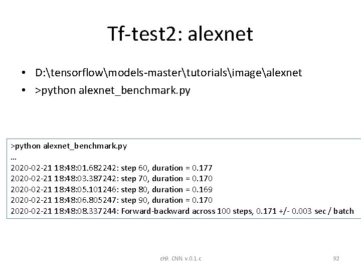
Tf-test 2: alexnet • D: tensorflowmodels-mastertutorialsimagealexnet • >python alexnet_benchmark. py … 2020 -02 -21 18: 48: 01. 682242: step 60, duration = 0. 177 2020 -02 -21 18: 48: 03. 387242: step 70, duration = 0. 170 2020 -02 -21 18: 48: 05. 101246: step 80, duration = 0. 169 2020 -02 -21 18: 48: 06. 805247: step 90, duration = 0. 170 2020 -02 -21 18: 48: 08. 337244: Forward-backward across 100 steps, 0. 171 +/- 0. 003 sec / batch ch 9. CNN. v. 0. 1. c 92

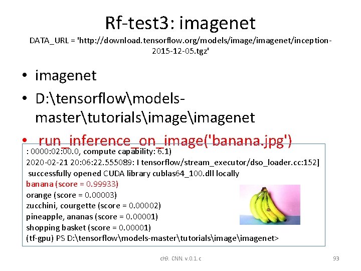
Rf-test 3: imagenet DATA_URL = 'http: //download. tensorflow. org/models/imagenet/inception 2015 -12 -05. tgz' • imagenet • D: tensorflowmodelsmastertutorialsimagenet • run_inference_on_image('banana. jpg') : 0000: 02: 00. 0, compute capability: 6. 1) 2020 -02 -21 20: 06: 22. 555089: I tensorflow/stream_executor/dso_loader. cc: 152] successfully opened CUDA library cublas 64_100. dll locally banana (score = 0. 99933) orange (score = 0. 00003) zucchini, courgette (score = 0. 00002) pineapple, ananas (score = 0. 00001) shopping basket (score = 0. 00001) (tf-gpu) PS D: tensorflowmodels-mastertutorialsimagenet> ch 9. CNN. v. 0. 1. c 93

Tf-test 4: cifar 10 object recognition of 10 classes • D: tensorflowmodelsmastertutorialsimagecifar 10? ? > ch 9. CNN. v. 0. 1. c 94

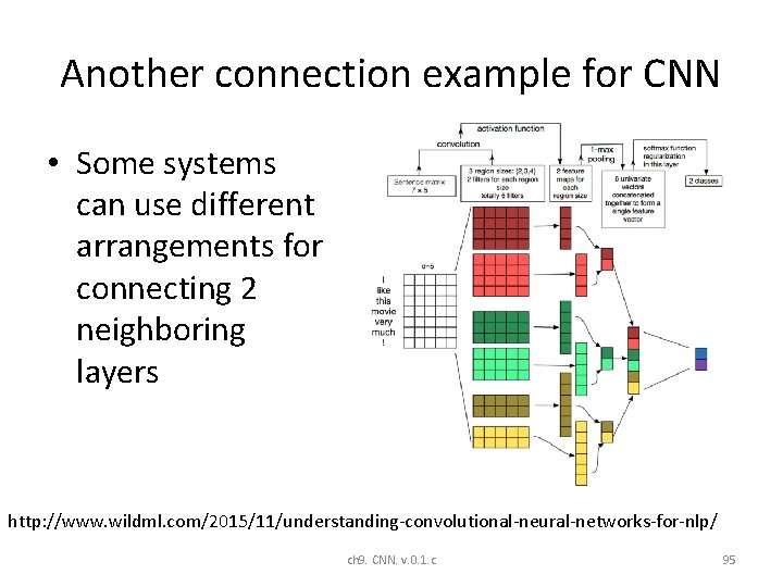
Another connection example for CNN • Some systems can use different arrangements for connecting 2 neighboring layers http: //www. wildml. com/2015/11/understanding-convolutional-neural-networks-for-nlp/ ch 9. CNN. v. 0. 1. c 95

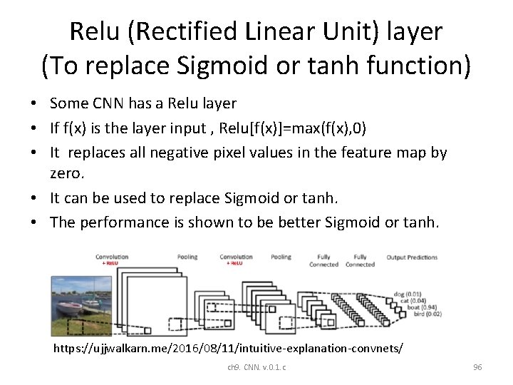
Relu (Rectified Linear Unit) layer (To replace Sigmoid or tanh function) • Some CNN has a Relu layer • If f(x) is the layer input , Relu[f(x)]=max(f(x), 0) • It replaces all negative pixel values in the feature map by zero. • It can be used to replace Sigmoid or tanh. • The performance is shown to be better Sigmoid or tanh. https: //ujjwalkarn. me/2016/08/11/intuitive-explanation-convnets/ ch 9. CNN. v. 0. 1. c 96

Answer : Exercises on CNN Exercise 1: Convolution (conv) layer How to find the curve feature • Exercise on convolution (implemented by correlation, see appendix). =C (empty cell = 0) A= 30 30 * 30 30 30 • • Find Y=correlation( A, C). If Y>5000, image A has feature C Answer: _____? =(30*50)+(30*50)=3000 (a bit small) What does the result of convolution( A, C) represent? Answer: That means the image in window A has no feature like C. ch 9. CNN. v. 0. 1. c 97

http: //deeplearning. stanford. edu/wiki/images/6/6 c/Convolution_schematic. gif , https: //link. springer. com/content/pdf/10. 1007%2 F 978 -3 -642 -25191 -7. pdf Answer 2: and Demo (click image to see demo) • 1 0 1 0 1 This is a 3 x 3 mask for illustration purpose, but noted that the above application uses a 5 x 5 mask. Input image A feature map X Y Convolution mask Exercise 2: (a) Find X, Y. Answer: X=____4 , Y=______3 (b) Find X again if the correlation mask is [0 2 0; 2 0 2; 0 2 0]. Answer: Xnew=2*1+2*1=6 ch 9. CNN. v. 0. 1. c A different kernel generates a different feature map 98

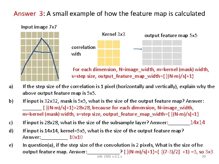
Answer 3: A small example of how the feature map is calculated Input image 7 x 7 Kernel 3 x 3 output feature map 5 x 5 correlation with For each dimension, N=image_width, m=kernel (mask) width, s=step size, output_feature_map_width={ [(N-m)/s]+1} a) b) c) d) e) If the step size of the correlation is 1 pixel (horizontally and vertically), explain why the above output feature map is 5 x 5. If input is 32 x 32, mask is 5 x 5, what is the size of the output feature map? Answer: _______ { [(N-m)/s]+1}=28 x 28, because for each dimension, N=image_width, m=kernel (mask) width, s=step size, output_feature_map_width={ [(N-m)/s]+1} If input is 28 x 28, what is the size of the subsample layer? Answer: ____14 x 14 If input is 14 x 14, kernel=5 x 5, what is the size of the output feature map? Answer: _____ 10 x 10 In question(a), if the step size of the convolution is 2 pixels, What is the size of he output feature map. Answer: ______? { [(N-m)/s]+1}={ [(7 -3)/2] +1) =3, so 3 x 3 ch 9. CNN. v. 0. 1. c 99