CH 9 Design via Root Locus 9 1

")
")


/S : PI controller → ess = 0 ( Proportional-plus-Integral)")

 1/S : idea integral compensator 理想積分器 →")


 = 1/(1 + Kp) = 0. 108 Kp =lims→")
 1/S : 4/11 idea integral compensator 理想積分器")

 = 1/(1 + Kp) = 0. 108 Kp = lims→")
 = 0. 0108 =")


 改變暫態反應 %OS不變 a. uncompensated; b.")


/(S+Pc) : Pc > Zc 設計目標: 補償後系統 %OS")


")


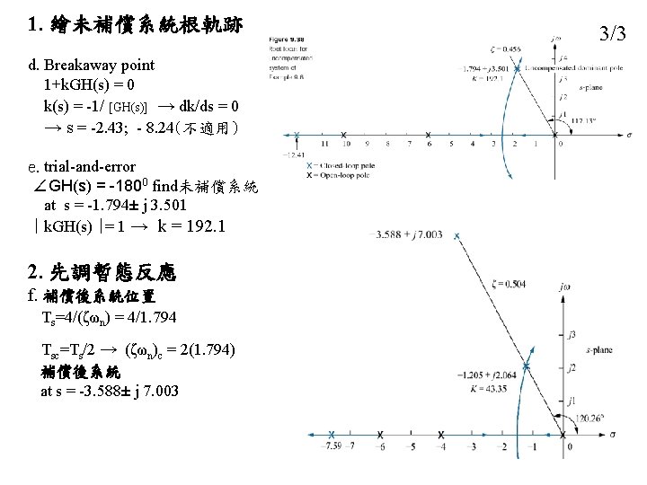
設計 補償後系統 at s = -3. 588± j")
= 192. 1/60 ess=1/Kv=60/192. 1 h.")
- Slides: 58
CH. 9 Design via Root Locus
9. 1 Introduction Figure 9. 1 a. possible design point via gain adjustment (A) design point that cannot be met via gain adjustment (B); 需補償器設計
9. 1 Introduction Figure 9. 1 a. possible design point via gain adjustment (A) design point that cannot be met via gain adjustment (B); Figure 9. 1 (b) responses from poles at A and B
補償器種類 Figure 9. 2 Compensation techniques: a. cascade; b. feedback
• 9. 2節: design of cascade compensation to improve ess • 9. 3節: design of cascade compensation to improve 暫態反應 • 9. 4節: design of cascade compensation to improve both ess and 暫態反應 • 9. 5節: design of feedback compensation
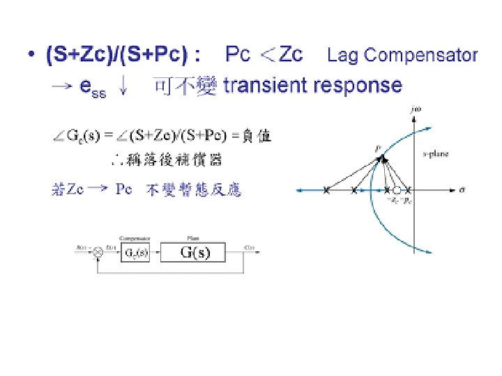
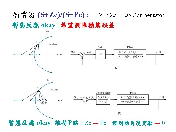
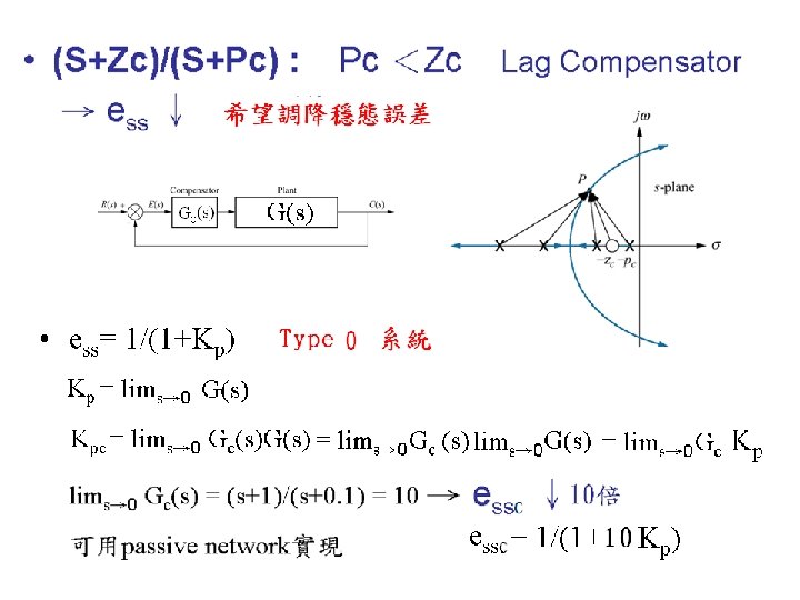
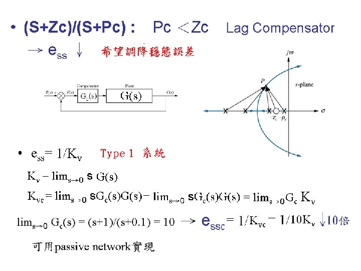
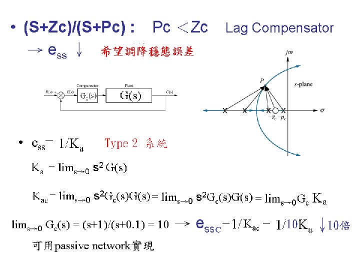
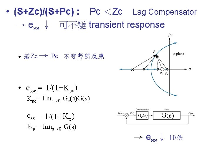
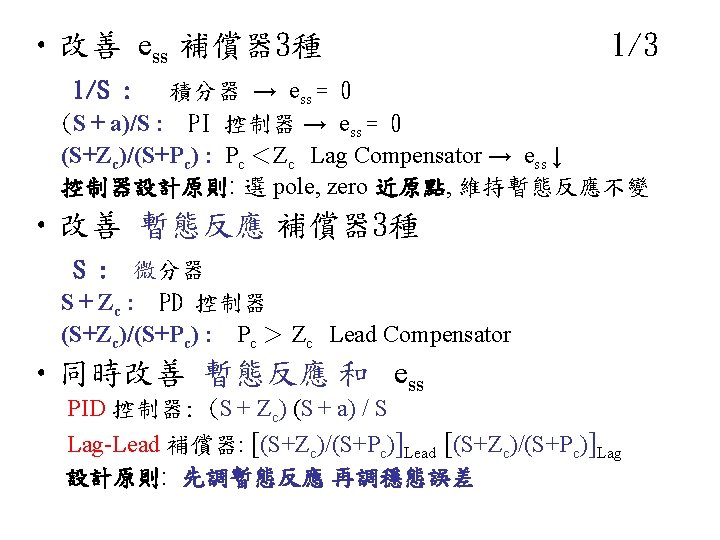
9. 2 cascade compensation to improve steady-state error • 改善 ess 補償器 3種 1/S : idea integral compensator 理想積分器 → ess = 0 亦變 transient response Fig. 9. 3 b (i. e. 變根軌跡圖) K 1 + K 2/S : PI controller → ess = 0 可不變 (S+Zc)/(S+Pc) : ( Proportional-plus-Integral) transient response Fig. 9. 3 c Pc <Zc Lag Compensator → ess ↓ 可不變 transient response
Figure 9. 3 a. root locus b. not on the root locus with 1/S compensator added 此設計已無從獲致系統 A
• 補償器 1/S : idea integral compensator → ess = 0 ∵ system type 增 1 ess = finite → ess = 0 (缺點 active network) (缺點 變transient response)
Figure 9. 3 c. on root locus with PI compensator added 當 a 甚小 → 0 不變 transient response PI controller 補償
• (S + a)/S : PI controller → ess = 0 ( Proportional-plus-Integral) ∵ system type 增 1 可不變 transient response 當 a 甚小 Fig. 9. 3 c (缺點 active network) (不變transient response)
Closed-loop system for Example 9. 1: 設計目標: 希望 ess = 0; 不變 transient response Figure 9. 4 (下頁說明控制器選擇) before compensation after PI compensation
• 改善 ess 補償器 3種 (控制器選擇) 1/S : idea integral compensator 理想積分器 → ess = 0 亦變 transient response Fig. 9. 3 b (i. e. 變根軌跡圖) K 1 + K 2/S : PI controller → ess = 0 可不變 (S+Zc)/(S+Pc) : ( Proportional-plus-Integral) transient response Fig. 9. 3 c Pc <Zc Lag Compensator → ess ↓ 可不變 transient response
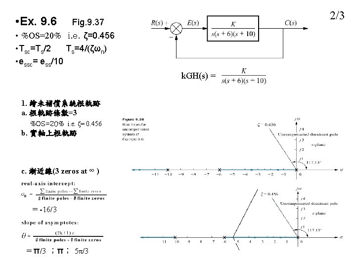
Example 9. 1 Figure 9. 5 Root locus for uncompensated system of Fig. 9. 4(a) 3階系統 Figure 9. 6 Root locus for compensated system of Figure 9. 4(b)
Figure 9. 7 time response PI compensated system response and the uncompensated system response of Example 9. 1 設計目標: ess = 0 不變 transient response
Figure 9. 8 PI controller
Uncompensated system 先畫根軌跡 找出系統現況 2/11
Uncompensated system 找未補償系統的穩態誤差 3/11 e(∞) = 1/(1 + Kp) = 0. 108 Kp =lims→ 0 G(s) =164. 6/20 = 8. 23
• 改善 ess 補償器 3種 (控制器選擇) 1/S : 4/11 idea integral compensator 理想積分器 → ess = 0 亦變 transient response Fig. 9. 3 b (i. e. 變根軌跡圖) K 1 + K 2/S : PI controller → ess = 0 可不變 (S+Zc)/(S+Pc) : ( Proportional-plus-Integral) transient response Fig. 9. 3 c Pc <Zc Lag Compensator → ess ↓ 可不變 transient response
5/11
Uncompensated system 7/11 e(∞) = 1/(1 + Kp) = 0. 108 Kp = lims→ 0 G(s) = 164. 6/20 = 8. 23 ec(∞) = 0. 0108 由Gc(s) 調整
Figure 9. 12 Compensated system of Figure 9. 11 ec(∞) = 0. 0108 = 1/(1 + Kpc) Kpc = lims→ 0 Gc(s)G(s) = lims→ 0 Gc(s) Kp = lims→ 0 Gc(s) 8. 23 = 91. 593 lims→ 0 Gc(s) = Zc/Pc = 11. 132 Gc(s) = (s+Zc)/(s+Pc) → 取 Pc=0. 01 → Zc=0. 111 8/11
Table 9. 1 9/11 Predicted characteristics of uncompensated and lagcompensated systems for Example 9. 2
Figure 9. 13 Step responses of uncompensated and lag-compensated systems for Example 9. 2 10/11
Figure 9. 14 Step responses of the system for Example 9. 2 lag compensator 更趨近原點 → 反應較慢 最終之ess不變 11/11
執行 Lag compensation 的相關公式
9. 3 Improving Transient Response via Cascade Compensation • 改善 暫態反應 補償器 3種 S : pure differentiator S + Zc : 純微分器 PD controller ( Proportional-plus-Derivative) (S+Zc)/(S+Pc) : Pc > Zc Lead Compensator 超前補償器
Figure 9. 15 Using PD compensation (S + Zc) 改變暫態反應 %OS不變 a. uncompensated; b. compensator zero at – 2; c. compensator zero at – 3; d. compensator zero at – 4 1/3
Figure 9. 16 time response 2/3 Uncompensated system and ideal derivative compensation solutions from Table 9. 2
Table 9. 2 Predicted characteristics for the systems of Figure 9. 15 3/3
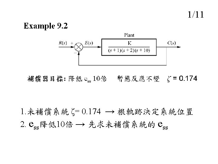
Example 9. 3 : S + Zc : PD controller Figure 9. 17 Feedback control system 1/7 設計目標: 補償後系統 %OS = 16% tsc = ts/3 i. e. ζ=0. 504
Figure 9. 18 Example 9. 3 Root locus for uncompensated system 先求未補償系統位置 %OS = 16% →ζ=0. 504 次求未補償系統 ts ts = 4/(ζωn) = 4/1. 205 = 3. 32 2/7
Figure 9. 18 Example 9. 3 Root locus for uncompensated system 2/7
Figure 9. 19 Compensated dominant pole superimposed over the uncompensated root locus for Example 9. 3 3/7 希望補償後 tsc= 3. 32/3 = 1. 107 → (ζωn)c = 3. 613 → %OS 不變 →補償後 dominant poles = -3. 613± j 6. 192 希望補償後 dominant poles = -3. 613± j 6. 192 設計 Gc(s) = S + Zc PD controller →∠Gc(s)G(s) = 1800 目標
Figure 9. 20 4/7 Evaluating the location of the compensating zero for Example 9. 3 希望之角度補償 ∠S + Zc = 1800 -∠G(s)
Figure 9. 21 Root locus for the compensated system of Example 9. 3 5/7
Figure 9. 22 time response Uncompensated and compensated system step responses of Example 9. 3 6/7
Table 9. 3 Uncompensated and compensated system characteristics for Example 9. 3 7/7
Figure 9. 23 PD controller S + Zc
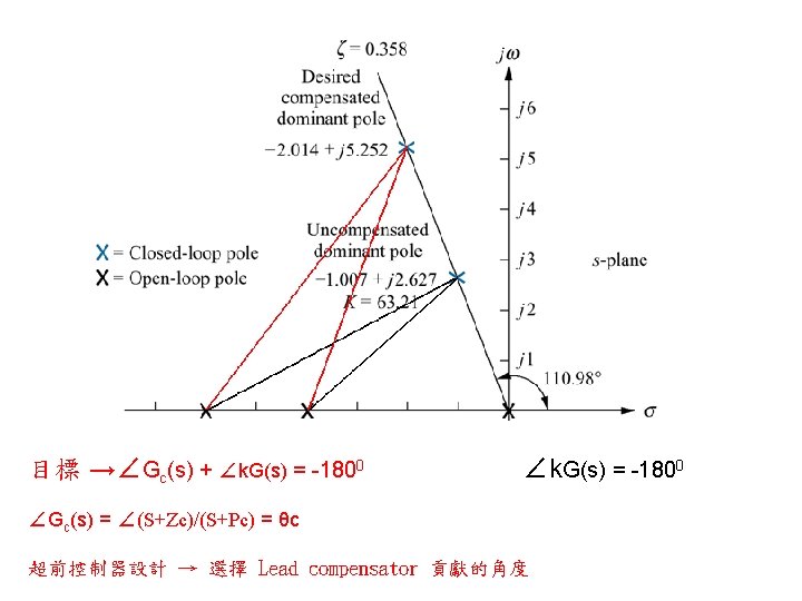
Example 9. 4 Lead compensator design (S+Zc)/(S+Pc) : Pc > Zc 設計目標: 補償後系統 %OS = 30% i. e. ζ=0. 358 tsc = ts/2 Figure 9. 26 uncompensated and compensated dominant poles
Figure 9. 25 Three of the infinite possible lead compensator solutions Lead compensator 貢獻的角度 (S+Zc)/(S+Pc) : Pc > Zc ∠(S+Zc)/(S+Pc) = θc 正值 超前控制器 目標 →∠Gc(s)G(s) = 1800 超前控制器設計 → 選擇 Lead compensator 貢獻的角度 → ∠Gc(s) = ∠(S+Zc)/(S+Pc) = θc
Table 9. 4 Comparison of lead compensation designs for Example 9. 4 Which is the best design? 系統階數? 是否有2個主要極點? 是否有零點? 能否抵消? 比較規格達成度 確認最佳設計
Figure 9. 28 Compensated system root locus (which is this design? )
Figure 9. 29 Uncompensated system and lead compensation responses for Example 9. 4
9. 4 design of cascade compensation to improve both ess and 暫態反應 • improve both 暫態反應 first • then improve ess • Example 9. 5 自修
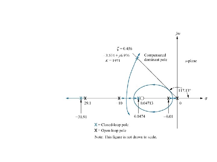
2. 先調暫態反應 g. Lead 補償器 Gc. L(s)設計 補償後系統 at s = -3. 588± j 7. 003 Gc. L(s) 角度貢獻 ∠Gc. LGH(s) = -1800 ∠Gc. L(s) = -1800 - ∠GH(s) = -1800 – (-164. 650) = - 15. 350 Gc. L(s)= (S+Zc)/(S+Pc) Pc > Zc 選 Zc = 6 → Pc = 29. 1 ∣k Gc. L(s)GH(s)∣= 1 → k = 1977 4/5
3. 後調穩態誤差 essc= ess/10 ess=1/Kv Kv=lims→ 0 sk. GH(s)= 192. 1/60 ess=1/Kv=60/192. 1 h. Lag 補償器 Gc. Lag(s)設計 經 Lead 補償後系統 at s = -3. 588± j 7. 003 Lag 補償器 需維持 system at s = -3. 588 ± j 7. 003 且降 essc= ess/10 = 60/1921 k Gc. Lag(s) Gc. LGH(s) Type 1系統 Gc. Lag(s)= (S+Zc)/(S+Pc) Pc <Zc i. e. Kvc=lims→ 0 s Gc. Lag(s) k. Gc. LGH(s) = 1921/60 lims→ 0 Gc. Lag(s) = (Zc/Pc )(1977/291) = 1921/60