CH 8 Nonparametric Methods Nonparametric methods do not

CH. 8: Nonparametric Methods Nonparametric methods do not assume a priori any model form. 8. 1 Nonparametric Density Estimation • Univariate case: Given the training set drawn iid from unknown probability density p(x) To estimate p(x),

• Cumulative distribution function (cdf): Density function (df): the derivative of the cdf

• Histogram estimator:

• Naive estimator: where weight function smooth spiky

8. 1. 1 Kernel Estimator • The above estimatiors are discrete. Kernel function: a smooth weight function, e. g. , Gaussian kernel: Kernel estimator (e. g. , Parzen windows)

6

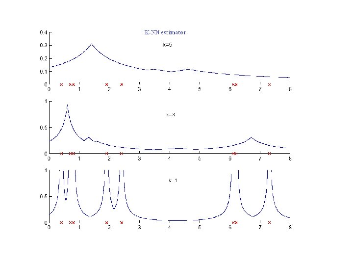
8. 1. 2 K-Nearest Neighbor Estimator • Instead of fixing h, fix # nearby examples K where the distance to the Kth closest example to x • The K-NN estimator is not continuous. To get a smooth estimator, a kernel function is used.

8. 1. 3 Generalization to Multivariate Data Kernel density estimator: and Multivariate Gaussian kernel: Euclidean form: Mahalanobis form:

8. 2 Nonparametric Classification The discriminant function: The continuous K-NN estimated class-conditional density: where The ML estimated prior density:

• The discrete K-NN estimation: # neighbors out of the K nearest The volume of hypersphere centered at x with radius , where is the kth nearest neighbor of x: with e. g. , as the volume of the unit sphere,

From Bayes’ rule: posterior probability K-NN classifier assigns the input to the class having most examples among the K neighbors of the input.

Example: 1 -NN classifier. It divides the space in the form of Voronoi tessellation. 8. 2. 1 Condensed Nearest Neighbor (CNN) Time/space complexity of K-NN is O(N). Idea: Find a subset Z of X that is small and is accurate in classifying X.

Algorithm of CNN: The algorithm depends on the order of the examples being examined; different subsets may be found.

The red line segments form the class discriminant. In the CNN, the examples that do not participate in defining the discriminant are removed.

8. 3 Nonparametric Regression: Regression problem: Given a training sample find . • Parametric method: Assume a model for , e. g. , a polynomial of certain order, and estimate the parameters of the model. • Nonparametric regression: Giving x, i) find its neighborhood N(x) and ii) average the r values in N(x) to calculate

There are various ways to defining the neighborhood and averaging in the neighborhood. In the following, consider univariate case. • Regressogram: Define a bin width, average the r values in the bin

• Running mean smoother: Define a bin symmetric around x and average in there • Kernel smoother: Give less weight to further points where K( ): Gaussian models

19

8. 4 How to Choose the Smoothing Parameters • Smoothing parameters: h: bin width, k: the number of neighbors. k or h large, many instances contribute to estimate, variance but bias (oversmoothing). k or h is small, variance is large, bias is small (undersmoothing).

8. 5 Outlier Detection • Outliers may reveal abnormal behaviors of systems. • Difficulties of outlier detection: outliers are very few and of many types. Idea -- find instances far away from other instances. Example: Local outlier factor (LOF) where the distance between x and its kth NN the neighborhood of x

LOF(x) 1, P(x not outlier) increases, larger, P(x outlier) increases.