Ch 7 Aggregate Demand Supply Aggregate supply Aggregate

Ch. 7: Aggregate Demand Supply –Aggregate supply –Aggregate demand –Macroeconomic equilibrium. –Effects of changes in aggregate supply and aggregate demand on economic growth, inflation, and business cycles –Explain U. S. economic growth, inflation, and business cycles by using the AS-AD model.

Aggregate Supply • Aggregate Supply Fundamentals – Long-run aggregate supply – Short-run aggregate supply

Aggregate Supply • Long-Run Aggregate Supply (LRAS) – relationship between the quantity of real GDP supplied and the price level when real GDP equals potential GDP. – Position of LRAS determined by • Labor supply • Labor demand • Production function

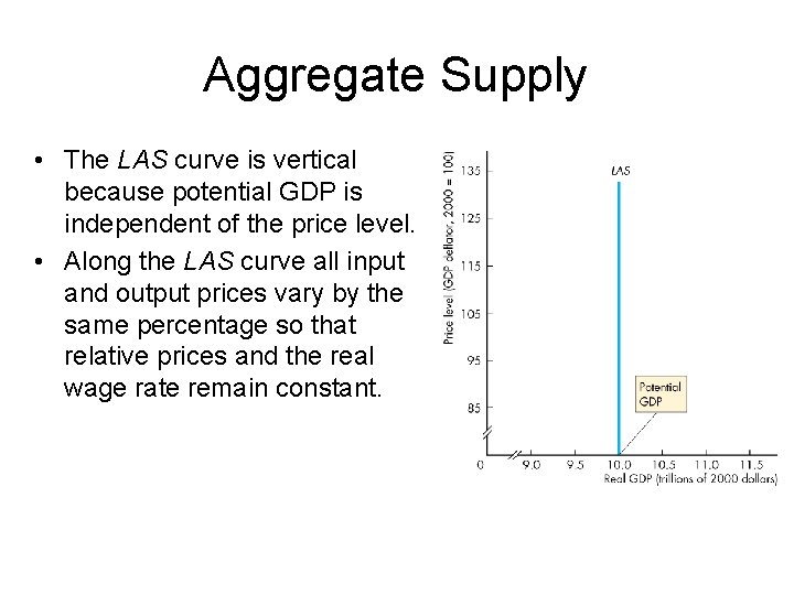
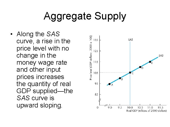
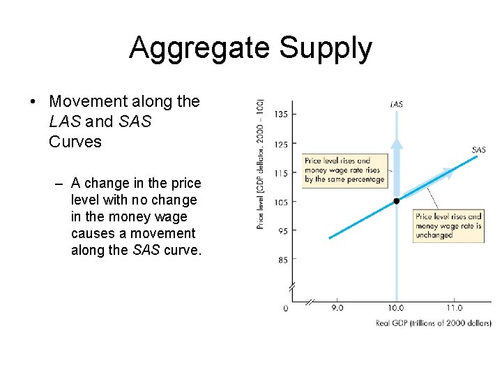
Aggregate Supply • The LAS curve is vertical because potential GDP is independent of the price level. • Along the LAS curve all input and output prices vary by the same percentage so that relative prices and the real wage rate remain constant.

Aggregate Supply • How will each of the following affect the position of the LAS curve? – increase in labor supply – Increase in labor demand – Upward shift of the production function

Aggregate Supply • Short-Run Aggregate Supply (SRAS) – The macroeconomic short run • a period during which some prices have not adjusted to the long run equilibrium • real GDP may fall below or rise above potential GDP. • the unemployment rate may rise above or fall below the natural unemployment rate. – SRAS is the relationship between the quantity of real GDP supplied and the price level in the short-run when the money wage rate, the prices of other resources, and potential GDP remain constant.

Aggregate Supply • Along the SAS curve, a rise in the price level with no change in the money wage rate and other input prices increases the quantity of real GDP supplied—the SAS curve is upward sloping.

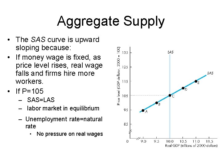
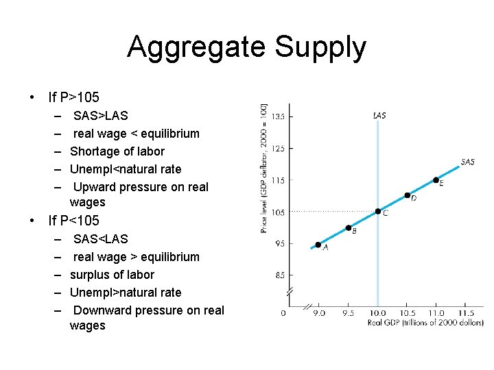
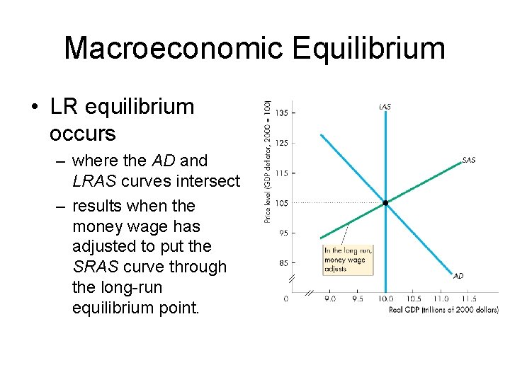
Aggregate Supply • The SAS curve is upward sloping because: • If money wage is fixed, as price level rises, real wage falls and firms hire more workers. • If P=105 – SAS=LAS – labor market in equilibrium – Unemployment rate=natural rate • No pressure on real wages

Aggregate Supply • If P>105 – – – SAS>LAS real wage < equilibrium Shortage of labor Unempl<natural rate Upward pressure on real wages • If P<105 – – – SAS<LAS real wage > equilibrium surplus of labor Unempl>natural rate Downward pressure on real wages

Aggregate Supply • Movement along the LAS and SAS Curves – A change in the price level with no change in the money wage causes a movement along the SAS curve.

Aggregate Supply • If real wage<equilibrium: – Real wages rise in long run – SAS shifts left • If real wage>equilibrium: – Real wages fall in long run – SAS shifts right

Aggregate Supply • Changes in Aggregate Supply – When potential GDP increases, both the LRAS and SRAS curves shift rightward. – Sources of change in Potential GDP • Change in the full-employment quantity of labor. • Change in the quantity of capital (physical or human). • Advance in technology.

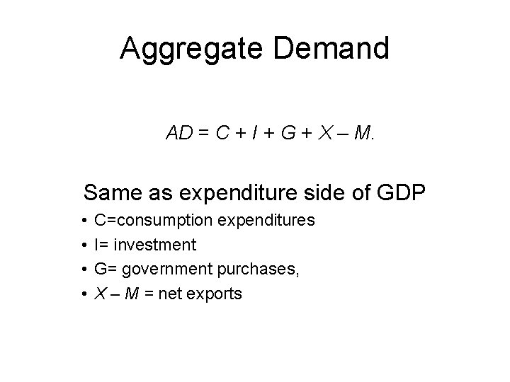
Aggregate Demand AD = C + I + G + X – M. Same as expenditure side of GDP • • C=consumption expenditures I= investment G= government purchases, X – M = net exports

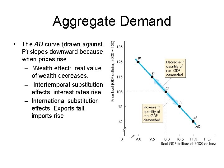
Aggregate Demand • The AD curve (drawn against P) slopes downward because when prices rise – Wealth effect: real value of wealth decreases. – Intertemporal substitution effects: interest rates rise – International substitution effects: Exports fall, imports rise

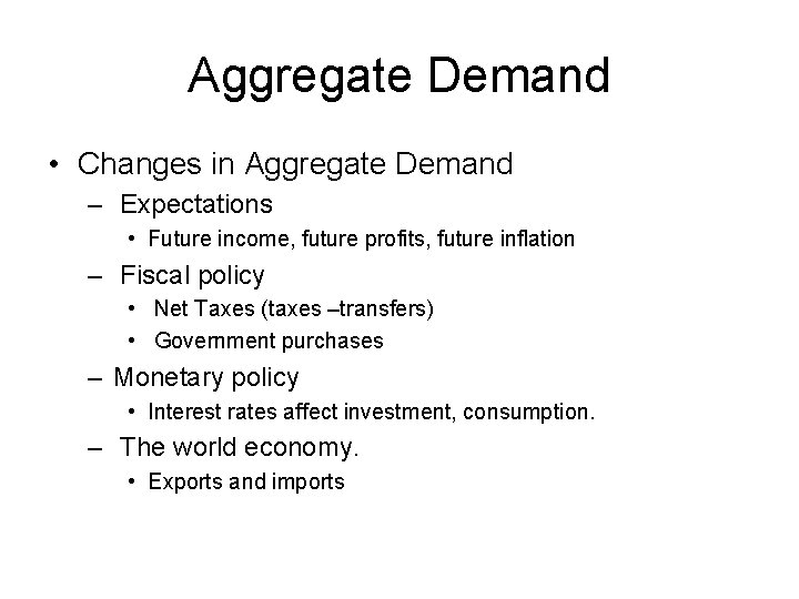
Aggregate Demand • Changes in Aggregate Demand – Expectations • Future income, future profits, future inflation – Fiscal policy • Net Taxes (taxes –transfers) • Government purchases – Monetary policy • Interest rates affect investment, consumption. – The world economy. • Exports and imports

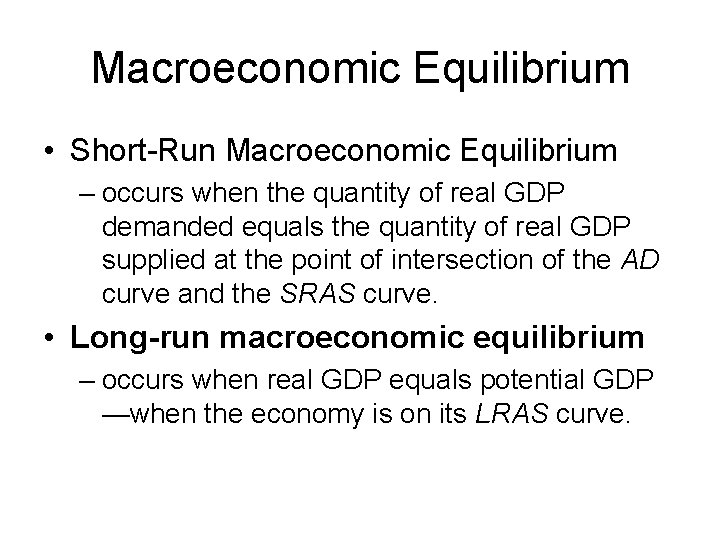
Macroeconomic Equilibrium • Short-Run Macroeconomic Equilibrium – occurs when the quantity of real GDP demanded equals the quantity of real GDP supplied at the point of intersection of the AD curve and the SRAS curve. • Long-run macroeconomic equilibrium – occurs when real GDP equals potential GDP —when the economy is on its LRAS curve.

Macroeconomic Equilibrium • LR equilibrium occurs – where the AD and LRAS curves intersect – results when the money wage has adjusted to put the SRAS curve through the long-run equilibrium point.

Macroeconomic Equilibrium • The Business Cycle – The business cycle occurs because AD and SRAS fluctuate but the money wage does not change rapidly enough to keep real GDP at potential GDP.

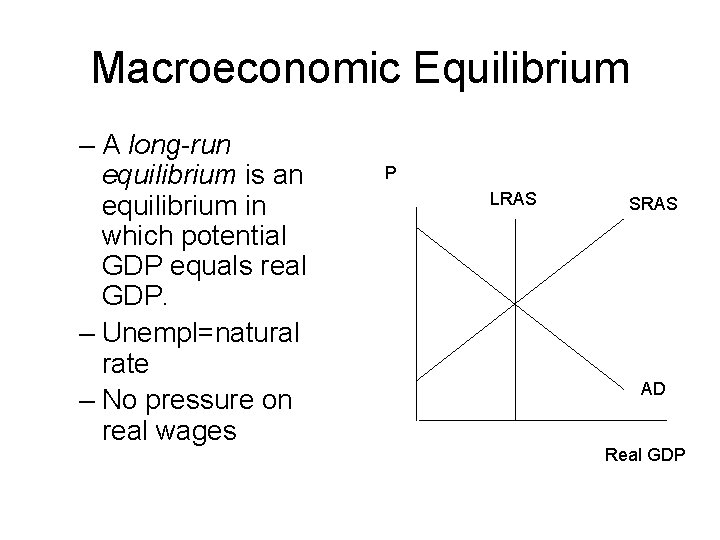
Macroeconomic Equilibrium – A long-run equilibrium is an equilibrium in which potential GDP equals real GDP. – Unempl=natural rate – No pressure on real wages P LRAS SRAS AD Real GDP

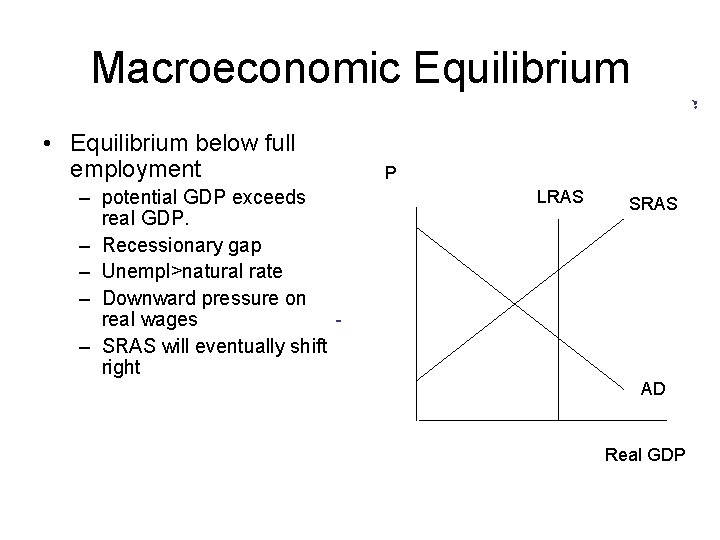
Macroeconomic Equilibrium • Equilibrium below full employment – potential GDP exceeds real GDP. – Recessionary gap – Unempl>natural rate – Downward pressure on real wages – SRAS will eventually shift right P LRAS SRAS AD Real GDP

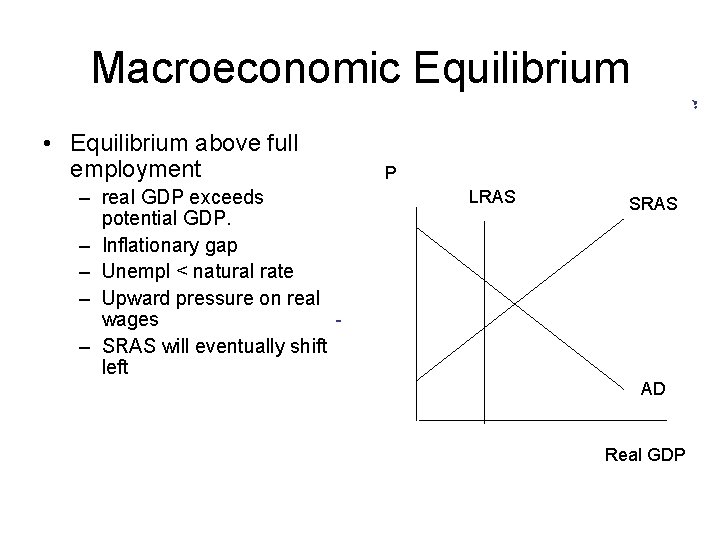
Macroeconomic Equilibrium • Equilibrium above full employment – real GDP exceeds potential GDP. – Inflationary gap – Unempl < natural rate – Upward pressure on real wages – SRAS will eventually shift left P LRAS SRAS AD Real GDP

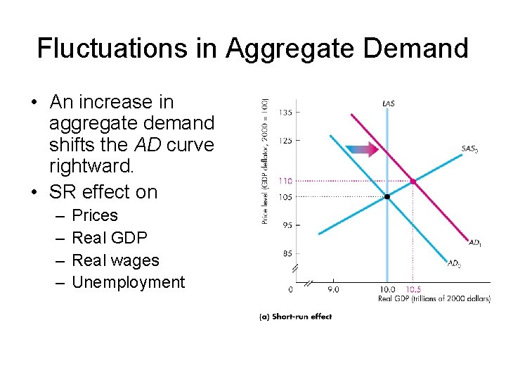
Fluctuations in Aggregate Demand • An increase in aggregate demand shifts the AD curve rightward. • SR effect on – – Prices Real GDP Real wages Unemployment

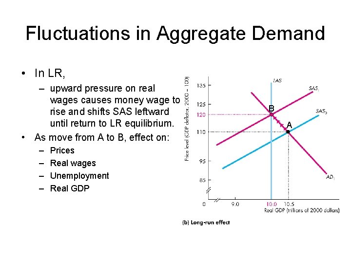
Fluctuations in Aggregate Demand • In LR, – upward pressure on real wages causes money wage to rise and shifts SAS leftward until return to LR equilibrium. • As move from A to B, effect on: – – Prices Real wages Unemployment Real GDP B A

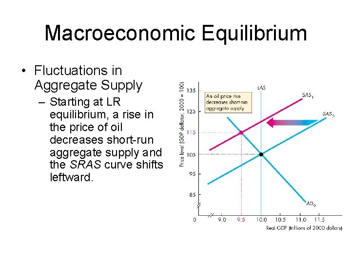
Macroeconomic Equilibrium • Fluctuations in Aggregate Supply – Starting at LR equilibrium, a rise in the price of oil decreases short-run aggregate supply and the SRAS curve shifts leftward.

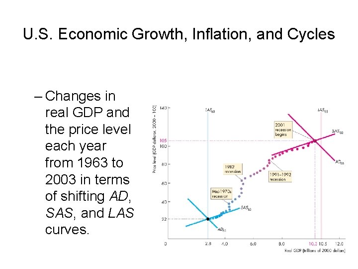
U. S. Economic Growth, Inflation, and Cycles – Changes in real GDP and the price level each year from 1963 to 2003 in terms of shifting AD, SAS, and LAS curves.

Using the AS/AD model • Starting from a LR equilibrium, examine the SR and LR effect of • Tax cut • Increase in government spending • Fed cuts interest rates • Consumer confidence rises • Temporary supply shock • Assume NO EFFECT on LRAS (to be considered later) • Variables to consider: • price, real wage, real GDP, unemployment.