CH 5 Reinforcement Learning 5 1 Introduction The

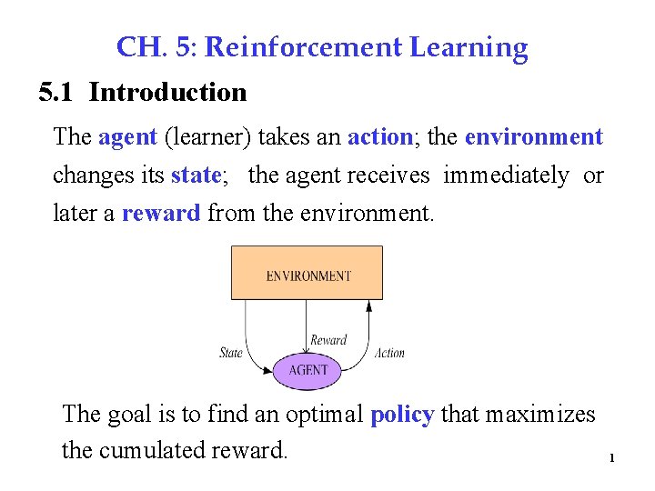
CH. 5: Reinforcement Learning 5. 1 Introduction The agent (learner) takes an action; the environment changes its state; the agent receives immediately or later a reward from the environment. The goal is to find an optimal policy that maximizes the cumulated reward. 1

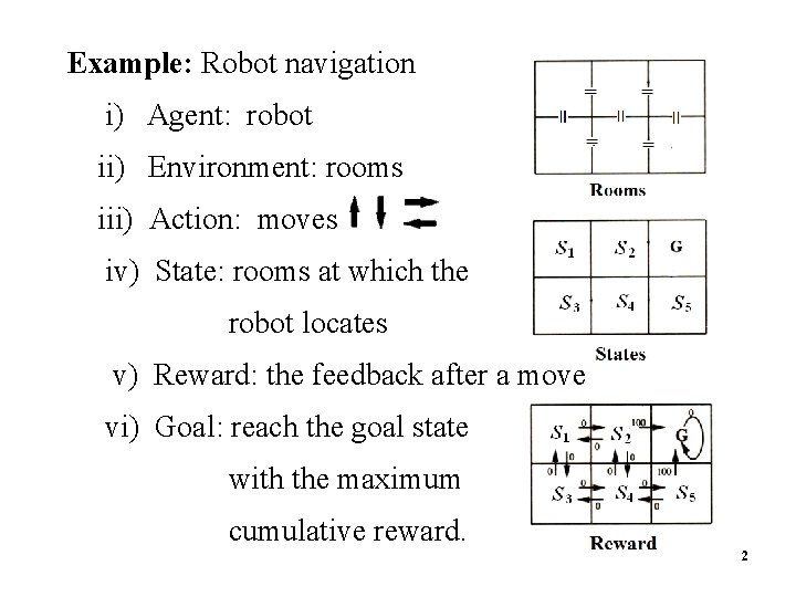
Example: Robot navigation 2 i) Agent: robot ii) Environment: rooms iii) Action: moves iv) State: rooms at which the robot locates v) Reward: the feedback after a move vi) Goal: reach the goal state with the maximum cumulative reward. 2

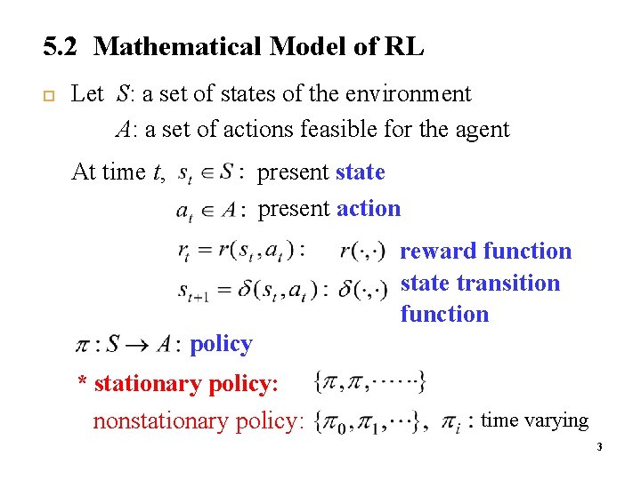
5. 2 Mathematical Model of RL Let S: a set of states of the environment A: a set of actions feasible for the agent present state present action At time t, reward function state transition function policy * stationary policy: nonstationary policy: time varying 3

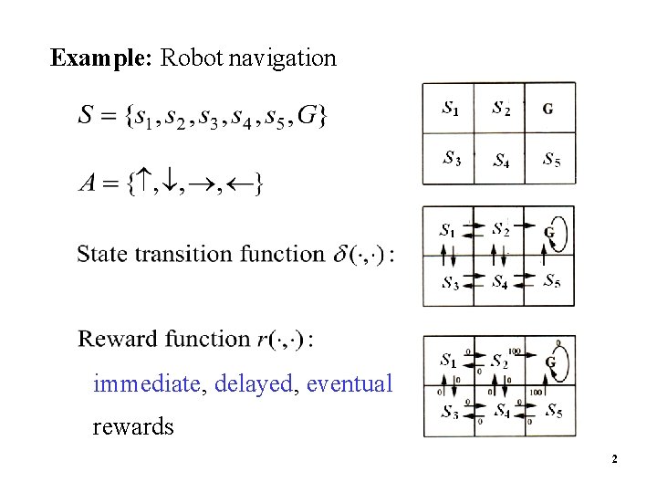
Example: Robot navigation immediate, delayed, eventual rewards 4 2

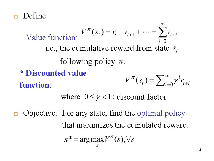
Define Value function: i. e. , the cumulative reward from state following policy * Discounted value function: . discount factor Objective: For any state, find the optimal policy that maximizes the cumulated reward. 4

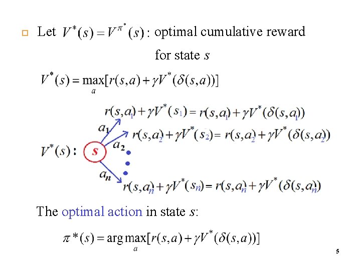
Let optimal cumulative reward for state s The optimal action in state s: 5

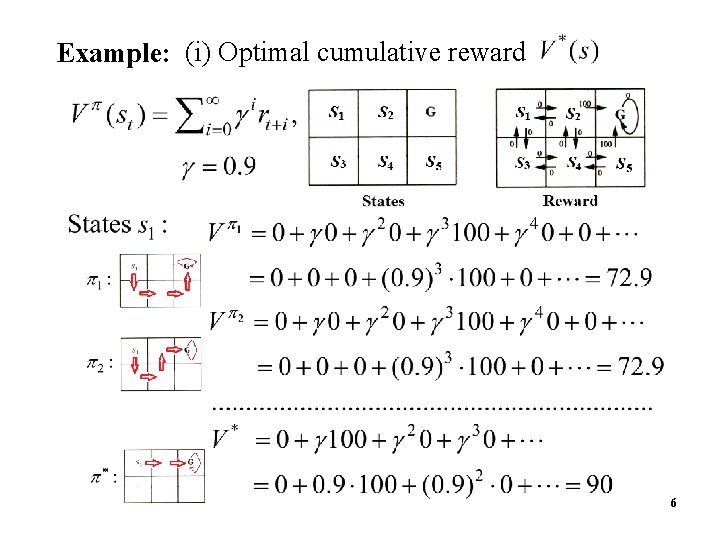
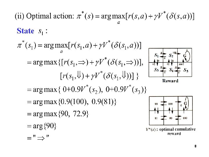
Example: (i) Optimal cumulative reward 6

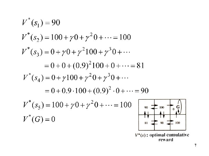
7

State 8

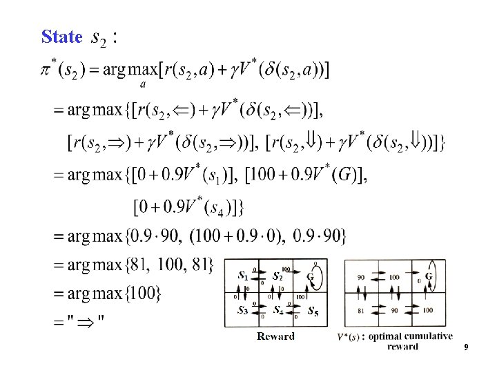
State 9

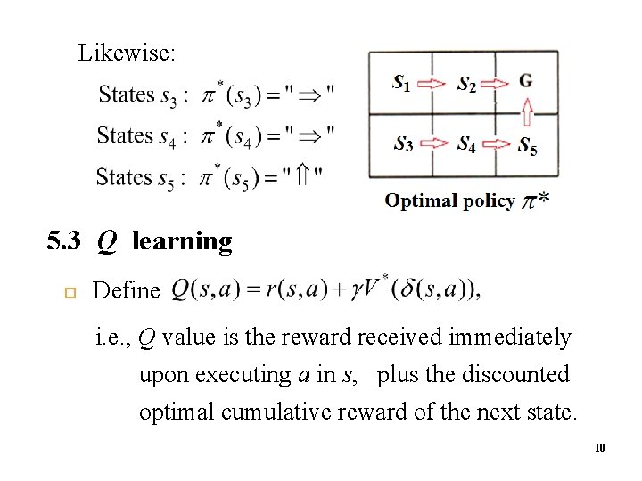
Likewise: 5. 3 Q learning Define i. e. , Q value is the reward received immediately upon executing a in s, plus the discounted optimal cumulative reward of the next state. 10

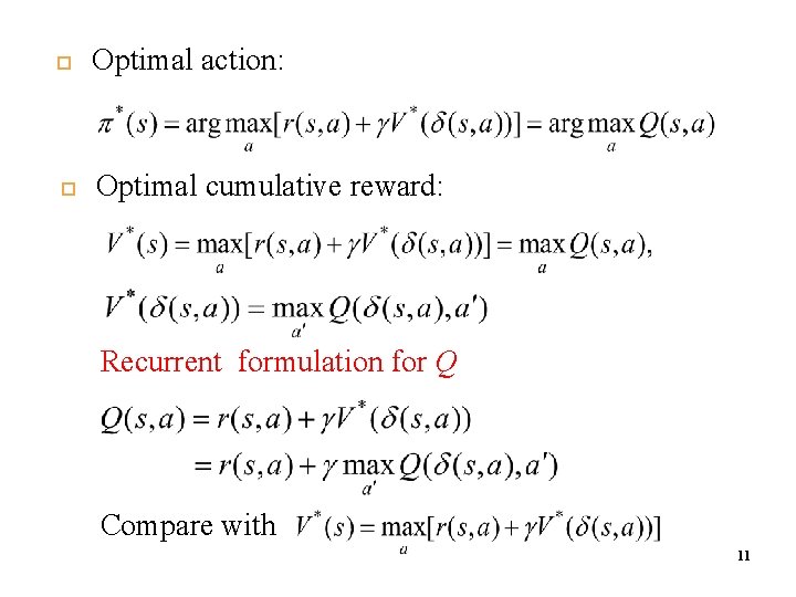
Optimal action: Optimal cumulative reward: Recurrent formulation for Q Compare with 11

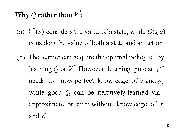
Why Q rather than (a) : considers the value of a state, while Q(s, a) considers the value of both a state and an action. (b) The learner can acquire the optimal policy learning Q or by . However, learning precise needs to know perfect knowledge of r and while good Q can be iteratively learned via approximate or even without knowledge of r and . 12

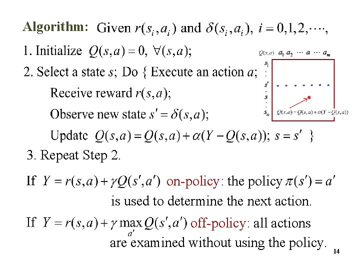
Algorithm: 3. Repeat Step 2. on-policy: the policy is used to determine the next action. off-policy: all actions are examined without using the policy. 14

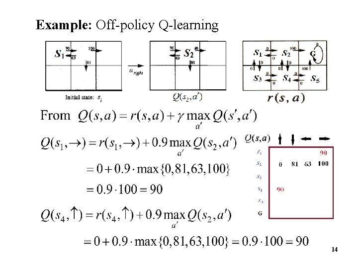
Example: Off-policy Q-learning 14

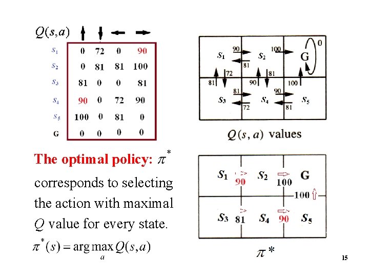
The optimal policy: corresponds to selecting the action with maximal Q value for every state. 15

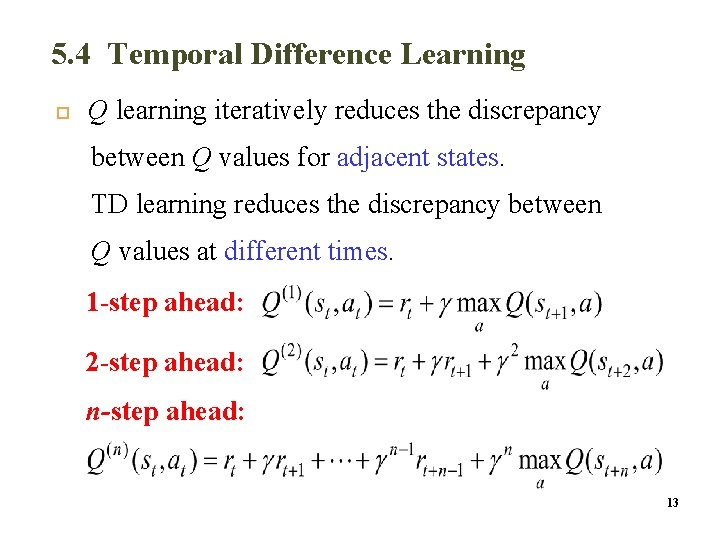
5. 4 Temporal Difference Learning Q learning iteratively reduces the discrepancy between Q values for adjacent states. TD learning reduces the discrepancy between Q values at different times. 1 -step ahead: 2 -step ahead: n-step ahead: 13

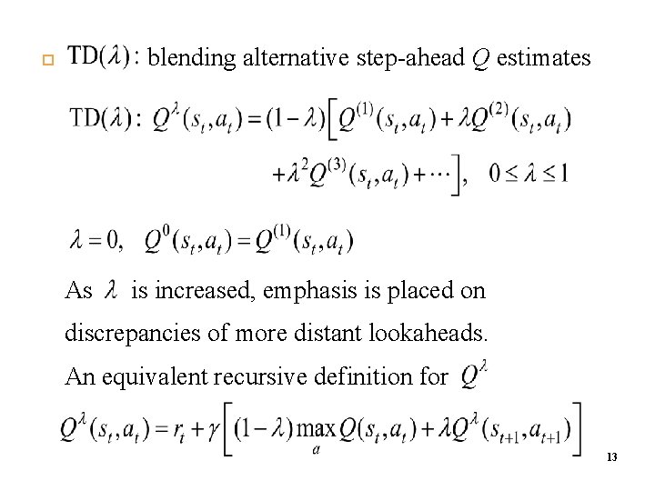
blending alternative step-ahead Q estimates As is increased, emphasis is placed on discrepancies of more distant lookaheads. An equivalent recursive definition for 13

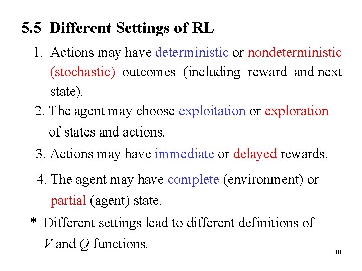
5. 5 Different Settings of RL 1. Actions may have deterministic or nondeterministic (stochastic) outcomes (including reward and next state). 2. The agent may choose exploitation or exploration of states and actions. 3. Actions may have immediate or delayed rewards. 4. The agent may have complete (environment) or partial (agent) state. * Different settings lead to different definitions of V and Q functions. 18