CH 405 Dynamics of Chemical Reactions Introduction to

CH 405 Dynamics of Chemical Reactions: Introduction to Modern Experimental Methods

Assessment methods Type of assessment Examinations Oral Presentation • Oral presentation 5 th December 9: 05 – 11: 55 B 209 Length 1. 5 Hours % weighting 80 20

Assessment methods ORAL PRESENTATION FOR CH 405 You have been given a research article or letter relating to material or techniques covered in the module. You are required to critically read the article and prepare a 10 minutes presentation for a non specialist audience, containing the following elements (in any order you deem appropriate): 1) The context of the article is explained 2) The main findings are described 3) The methodology used by the investigators is outlined 3 -4 minutes of discussion (based on questions asked to you by lecturers or other students) will follow your presentation. You should be able to provide clarification on any aspect you decided to include in the presentation.

5 lectures VGS • The LASER and its properties • Laser based techniques • Examples of modern techniques through pioneering studies: Photodissociation: – Femtochemistry – High Rydberg Time of Flight

The LASER Reminder Light: • Electromagnetic radiation • Sinusoidally oscillating electric and magnetic fields

LASER light – Special properties Light Amplification by the Stimulated Emission of Radiation • • • High directionality High intensity Can be highly monochromatic Can be continuous or very short pulsed Highly polarised (all E vectors aligned)

Interaction of light / matter Absorption E 2 n 2 E 1 n 1 • Photon lost • Sample absorbs energy Rate of absorption ρ(ν)n 1 Rate of absorption = B 12ρ(ν)n 1 B 12 is the Einstein coefficient for absorption

Interaction of light / matter Spontaneous Emission E 2 n 2 • Photon created • Sample emits (loses) energy E 1 n 1 Rate of spontaneous emission n 2 Rate of spontaneous emission = A 21 n 2 A 21 is the Einstein coefficient for spontaneous emission

Interaction of light / matter Stimulated Emission • Photon created • Sample emits (loses) energy • The stimulated emission is monochromatic and in phase with the same polarization as the stimulating photon E 2 n 2 E 1 n 1 Rate of stimulated emission ρ(ν)n 2 Rate of stimulated emission = B 21ρ(ν)n 2 B 21 is the Einstein coefficient for stimulated emission

Einstein coefficients: It can be shown that actually there is only one independent Einstein coefficient: At eqm, rate absn = rate st. em + rate sp. em B 12ρ(ν)n 1 = B 21ρ(ν)n 2 + A 21 n 2 i. e. , ρ(ν) = A 21 B 12 ehν/kt - B 21 n 2 -ΔE/kt Recall = e n 1 1 Yet Planck’s law states ρ(ν) = 8πhν 3. eh ν /kt -1 c 3 i. e. , B 21 = B 12 = CA 21 LASER radiation is dominated by stimulated emission

Conditions for LASER Action • Stimulated emission to dominate spontaneous emission • Want more photons out than are absorbed • Feedback • Amplification in a fixed direction

These impose requirements : A) If stim. Emission is to dominate absorption, we need rate of stim. Emission >> rate of absorption B 21ρ(ν)n 2 >> 1 B 12ρ(ν)n 1 i. e. , n 2 >> 1 n 1 But for systems in equilibrium, n 2/n 1 is given by the Boltzmann Law: which for all temperatures gives n 2 < n 1. ( kt n 2 g 2 e = n 1 g 1 In other words we require population inversion -ΔE ( i. e. ,

Other requirements : B) If Stim. Emission is to dominate spontaneous emission, we need rate of stim. Emission >> rate of spont. emission i. e. , B 21ρ(ν)n 2 >> 1 A 21 n 2 i. e. , B 21 ρ(ν) >> 1 A 21 We require the radiation intensity to be as large as possible.

Partial mirror 100% Reflective mirror Typical LASER cavity Lasing medium (gas, crystal etc. )

Schematic LASER Action Partial mirror 100% Reflective mirror 1: Pump system to excited levels

Schematic LASER Action Partial mirror 100% Reflective mirror 2: Initial spontaneous emission

Schematic LASER Action Partial mirror 100% Reflective mirror 3: Followed by stimulated emission

Schematic LASER Action Partial mirror 100% Reflective mirror 4: Feedback produces amplification – light leaks out of the partial mirror each trip

Specific Examples of lasers Different Lasers have: • Different lasing media • Different, often sophisticated methods of generating population inversion Some are fixed wavelength – others tuneable.

A. The Helium Neon Laser • Very common • A gas laser (medium a mixture of He and Ne) • The first continuous wave (cw) laser • Lasing occurs in excited Ne atoms • Most common wavelength 632. 8 nm (RED)

He. Ne Discharge creates metastable, He* +Ne Ne* + He Creates population inversion in Ne He Ne

B. The excimer / exciplex laser • Gas lasers • Electric discharge creates ions which recombine to give exotic species (excited dimers) • Usually high energy pulsed lasers (up to 1 J/10 ns) • Almost always generate ultraviolet light • Common versions include • Ar. F (193 nm) produces O 3 in lab-pungent • Kr. F (248 nm) • Xe. Cl (308 nm) Very common

• Discharge ionizes gas mix • Ar+ and F- recombine on excited ionic surface • Upon charge transfer the system drop to the covalent surface which is dissociative – always population inversion l co li o si n Discharge / reaction Excimers

C. The Nd: YAG LASER • Solid state laser (crystalline rods) • Nd 3+ ions doped in a Yttrium Aluminium Garnate crystal • Population inversion achieved by external pumping with flashlamps • Can be cw or pulsed • Lases at 1064 nm (near IR) but frequency doubling generates harmonics at 532 nm or 355 nm.

Tuneable Lasers: Dye Lasers • Use large organic molecules as lasing medium • Population inversion is created by pumping with a fixed wavelength laser (e. g. , excimer / Nd. YAG) • Each dye has a tuning window determined by its fluorescence spectrum. • Dye has a lifetime. Need to replace every so often (Rhodium 6 G very popular-Red).

Schematic dye laser Pump laser Partial mirror q Diffraction grating Organic Dye solution

Common dye: Rhodamine 6 G LASE PUMP

Different dyes cover IR-UV

Ultrafast lasers ps ns 10 -9 s 10 -12 s time fs 10 -15 s

Generating ultrafast laser pulses Mode locking-Revision This technique can produce pulses of picosecond (1 ps = 1 x 10 -12 Sec) duration and less. The laser radiates at a number of different frequencies depending on (a) the medium and (b) the number of half wavelengths trapped between the mirrors (resonant modes) nx 1 λ = L 2 n = Integer L = Length of cavity Locking the phases of the different frequencies together, interference leads to a series of sharp peaks (pulse duration).

Intensity Generating ultrafast laser pulses Doppler profile of gain medium Δν Resonant modes (there are N of these) Full width half maximum (FWHM) ~ N(7) x Δν Frequency (ν) By locking the phases of the modes and allowing them to interfere, the point of constructive interference corresponds to the laser pulse output. The more nodes present, the shorter the pulse in time (frequency-time uncertainty).

Generating ultrafast laser pulses The resonant modes differ in frequency (ν) by c Δv = 2 x. L Δt = c = speed of light 1 N = resonant modes N x Δν For example, for a FWHM of 200 cm-1 and a 1 meter length cavity, this leads to 40000 resonant modes and a pulse duration of 0. 17 ps or 170 femtoseconds (1 fs = 10 -15 Sec).

Generating ultrafast laser pulses The example given is for equal mode amplitudes. In reality, this is not true. For example, a laser producing pulses with a Gaussian temporal shape gives: 0. 441 N = resonant modes Δt = N x Δν Therefore, for a FWHM of 200 cm-1 and a 1 meter length cavity, the pulse duration becomes 0. 07 ps or 73. 5 fs

Generating ultrafast laser pulses Active mode locking Involves the periodic modulation of the cavity loss or the round trip phase change with an acousto-optic modulator. If the modulation is synchronized with the cavity round trips, this leads to generation of ultrafast pulses, normally picosecond duration. Passive mode locking Involves the generation of much shorter pulses (femtoseconds) and relies on the optical Kerr effect in which the refractive index of the gain medium (say Ti. Sapphire) changes when exposed to intense electric fields. The cavity loss is modulated much faster than with an electronic modulator (e. g. acousto-optic).

Example: Spitfire® XP ‘Seed’ laser Amplifier

Outline • Background on regenerative amplification – Intro – Comparison Multipass vs Regen • Spitfire Pro features and performances – Optical layout – Stretcher/compressor – Regen cavity

Regenerative Amplification • Goal: amplify ultra-short pulses (20 fs-100 ps, n. J, tens of MHz) up to the milli Joule level • Motivation: need for ultra-short, high peak power, frequency tunable pulses for: – Scientific research (spectroscopy, pump-probe, non linear physics) – Industrial and scientific micro/nano-machining • Gain medium: Titanium: Sapphire (Ti: Sapphire) – Large gain bandwidth (650 -1100) supports ultra short pulses down to 10 fs, large tunability throughout the gain range – High thermal conductivity facilitates rod thermal management at high pump power

Regenerative Amplification Amplify ~12 ns Time (μs) 82 MHz seed (from modelocked output) amplified at 1 k. Hz (typically) in a regenerative amplifier

Regenerative Amplification General scheme: 1. Trap seed pulse in an optical cavity 2. Pass pulse multiple times through Ti: Sapphire rod until amplified to desired energy level 3. Switch pulse out – – But with short high energy pulses there is risk of damage and self-focusing in the Ti: Sapphire rod. Need to maintain a low peak power in critical components of the system. Chirped Pulse Amplification (CPA)

Chirped Pulse Amplification Stretch in time = Chirp = introduce GVD Frequencies are: 1. spread in time (x 104) 2. safely amplified at different times in the rod 3. Recombined to form a short amplified pulse Pulse from seed laser (Tsunami or Mai Tai) A few 10 s fs stretcher Stretched pulse A few 100 ps Output Pulse from Spitfire A few 10 s fs Amplified Pulse amplifier compressor

The system layout (DNL) M PD Faraday isolator M Iris M M M Stretcher grating Compressor grating M CM PC 2 M M PD L L M M Ti: Sapphire Rod M M PC 1 TFP M M L M M M

Enhanced Spitfire XP Regen Cavity (DNL) Patented single Pockels cell cavity design: less material dispersion → shorter pulse width normal incidence rod → higher power and better mode The Spitfire Pro XP is specified at <35 fs and >3. 5 W M 1 Rod TFP PC 2 W P Intra-cavity components: M 1, M 2 : End mirrors Rod : Ti: Sapphire rod WP : ¼ Waveplate TFP : Thin Film Polarizer PC 2 : Pockels Cell M 2

Enhanced Spitfire XP Regen Cavity (DNL) Regen Operation: Before Injection Only the pulse to be amplified enters the cavity Seed input M 1 TFP P C 1 Rod TFP PC 2 W P Intra-cavity components: M 1, M 2 : End mirrors Rod : Ti: Sapphire rod WP : ¼ Waveplate TFP : Thin Film Polarizer PC 2 : Pockels Cell M 2

Enhanced Spitfire XP Regen Cavity (DNL) Regen Operation: PULSE Injection Pulse is injected using the external Pockels cell PC 1. Pulse is trapped using the internal Pockels cell PC 2. Seed input M 1 TFP P V 1=Vl/2 C 1 Rod TFP PC 2 W P Intra-cavity components: M 1, M 2 : End mirrors Rod : Ti: Sapphire rod WP : ¼ Waveplate TFP : Thin Film Polarizer PC 2 : Pockels Cell M 2 V 2=Vl/4

Enhanced Spitfire XP Regen Cavity (DNL) Regen Operation: Pulse AMPLIFICATION Seed input M 1 TFP P C 1 Rod TFP PC 2 W P Intra-cavity components: M 1, M 2 : End mirrors Rod : Ti: Sapphire rod WP : ¼ Waveplate TFP : Thin Film Polarizer PC 2 : Pockels Cell M 2 V 2=Vl/4

Enhanced Spitfire XP Regen Cavity (DNL) Regen Operation: Pulse EJECTION Internal Pockels cell PC 2 is turned off output Seed input M 1 TFP P C 1 Rod TFP PC 2 W P Intra-cavity components: M 1, M 2 : End mirrors Rod : Ti: Sapphire rod WP : ¼ Waveplate TFP : Thin Film Polarizer PC 2 : Pockels Cell M 2 V 2=Vl/4 V 2=0

Enhanced Spitfire XP Regen Cavity (DNL) Patented single Pockels cell cavity design: less material dispersion → shorter pulse width normal incidence rod → higher power and better mode The Spitfire Pro XP is specified at <35 fs and >3. 5 W M 1 Rod TFP PC 2 W P Intra-cavity components: M 1, M 2 : End mirrors Rod : Ti: Sapphire rod WP : ¼ Waveplate TFP : Thin Film Polarizer PC 2 : Pockels Cell M 2

Switching out cavity Without switching With switching

Frequency doubling As e-m radiation passes through a medium it sets up a polarization in the medium, P given by the series: P = ε 0(χ(1) E + χ(2) E 2 + χ(3) E 3 + …) where χ(i) is the ith order susceptibility and E is the electric field. Most optical phenomena (e. g. reflection) can be understood in terms of χ(1). However, at high electric field intensities, the non-linear terms (χ(2) and χ(3)) become significant. Consider a light wave of the form: E = E 0 sin(ωt)

Frequency doubling cont. The polarization thus becomes: P = ε 0χ(1)E 0 sin(ωt) + ε 0χ(2)E 02 sin 2(ωt) + ε 0χ(3)E 03 sin 3(ωt) + …) P = ε 0χ(1)E 0 sin(ωt) + (ε 0χ(2)/2)E 02 (1 -cos(2ωt)) + (ε 0χ(3)/4)E 03(3 sin(ωt) - sin(3ωt) + …) 2 x orig frequency (SHG) SHG achieved in crystals with no center of symmetry l 1 l 1/2

Other (non-laser) light sources Optical parametric oscillators use non-linear optics in a different way to split high energy (e. g. , UV) photons into two lower energy photons (one visible, one infra-red) subject to conservation of energy. l 2 l 1 l 3 Synchrotron sources are national facilities producing enormously tuneable (and very high energy) radiation generated by the acceleration of charged particles, e. g. , electrons, around enormous storage rings. They produce weak fluences but are the most common sources* of tuneable hard X-ray and XUV.

LASER Applications in Chemical Physics Reading: Gardner & Miller, J. Chem. Phys. 121, 5920, (2004)

By way of illustration we will concentrate on two types of application: A. Determining Quantum state distributions of a sample: Laser Induced Fluorescence (LIF) Resonance Enhanced Multiphoton Ionization (REMPI) B. Determining kinetic energy (or mass/velocity) distributions of a sample: Laser Ionization Time Of Flight Mass-Spec (LI TOFMS) There are, of course a plethora of other laser applications but these will prove useful later when we examine real examples.

So how does one determine the quantum state distribution of a sample? Almost always by some form of spectroscopy – i. e. , exciting transitions between different: And electronic, X, A, B, Σ, Π vibrational, v, or (v 1, v 2, v 3) rotational, J, or JKa, Kc quantum states And why would one want to? The quantum state distribution gives us information on the internal energy of the molecules in a sample (i. e. , large amounts of electronic and/or vibrational and/or rotational excitation).

A. Laser Induced Fluorescence (LIF) A system in an electronically excited state can decay back to a lower lying state by emitting a photon. Detection of the photons can be used to infer information on the state distribution. • Excite sample with a pulsed tuneable (UV) laser. • Photons emitted only when the laser is resonant with a transition from an occupied level to an excited level. • Can achieve rotational resolution for small molecules, vibrational resolution for larger molecules + simple (1 - photon) spectra, large signals, lifetime information - Not all states fluoresce (not universal), collection efficiency poor, need to know excited states

2 variants of LIF: Total Fluorescence (or fluorescence excitation) detector scan l • Collect all light emitted as a function of excitation λ. • Info on excited states from line positions and • Info on ground state populations from spectral intensities.

Fluorescence excitation spectrum of jet-cooled (5 K) toluene E→

Vibrations of ground state benzene Sym. Species a 1 g a 2 g a 2 u b 1 u b 2 g b 2 u e 1 g e 1 u e 2 g e 2 g e 2 u No 1 2 3 4 5 6 7 8 9 10 11 12 12 13 14 15 16 16 17 18 19 20 20 Approximate type of mode CH str Ring str CH bend CH str Ring deform CH bend Ring deform Ring str CH bend CH str Ring str + deform CH bend CH str Ring str CH bend Ring deform Selected Freq. Value (cm-1) 3062 992 1326 673 3068 1010 995 703 1310 1150 849 3063 1486 1038 3047 1596 1178 606 975 410

HS fragments produced in 248 nm photodissociation of H 2 S Rotational Resolution A 2Σ(v=0, J)←X 2Π(v=0, J) P 21 Intensity / arbitrary units 19/2 P 11 1/2 15/2 1/2 Q 11 3/2 15/2 R 12 Q 22 13/2 7/2 R 11 Q 21 1/2 21/2 P 22 3/2 Q 12 P 12 1/2 R 21 3/2 R 22 1/2 30400 15/2 13/2 30600 Wavenumber / cm 30800 -1 31000

Vibrationally excited HCO produced in the O (3 P) + C 2 H 4 → HCO + CH 3 reaction B←X transition (v 1, v 2, v 3) v 1= C-H stretch v 2 Mixed bending v 3 and C-O stretch Gardner & Miller, J. Chem. Phys. 121, 5920, (2004)

Dispersed Fluorescence • Fix excitation λ to excite a single (ro)vibrational transition • Disperse the fluorescence (using a monochromator) to determine the individual wavelength components. • Learn about ground state levels

Fluorescence excitation spectrum of ethoxy radical Dispersed Fluorescence (from 1003)

B. Resonance Enhanced Multiphoton Ionization (REMPI) Instead of trying to detect photons (which are emitted in all directions and can only be detected with ~10% efficiency) it is more efficient (although harder) to detect ions produced by photoionization of the sample molecules. Typical small molecule ionization energy ~10 e. V i. e. , require a photon of λ < 125 nm (deep UV) - very difficult to generate in the laboratory. Instead use simultaneous absorption of several photons to ionize the atom/molecule/cluster.

REMPI (cont. ) Take advantage of the fact that the probability of ionization is enormously enhanced if the photons are resonant at the n photon level with an excited state AB*. energy IP AB+ + e- AB* 2+1 REMPI AB • Excite with tuneable pulsed laser • AB→→AB*→AB+ + e • Detect ions only when laser is resonant with excited state + 100% efficient ion detection, ionization is universal, can access unusual states, high species selectivity - Need powerful lasers (£££), complicated selection rules, intermediates often not characterised

REMPI of N 2 from 193 nm dissociation of N 2 O 57% excess energy appears in rotation N 2 O 193 nm → N 2 + O N 2 X 1Σg+ →→ a’’ 1Σg+(v=0, J )→ N 2+

Mass / Kinetic Energy Determination E Flight distance, L + m 3 + HV 0 V + m 2 m 1 < m 2 <m 3 + m 1 detector Laser ionization time-of-flight (TOF) mass spectrometry m 2 m 3 m 1 time • Laser pulse ionizes sample (t=0), ions are accelerated in electric field (to HV/2 if laser hits the centre) • All ions leave with the same kinetic energy: ½ m 1 v 12 = ½ m 2 v 22 = ½ m 3 v 32 • The arrival time at the detector, t, depends only on v: t i ≈ L/vi • Hence singly charged ions are separated according to their mass.

Mass Determination Using a known mass to predict an unknown mass: Time-of-flight (μs) ? (4. 24μs) m 1 = m 2 ? (4. 12μs) H (1μs) Intensity (arb. units) d V= t t 1 t 2 2 ( ) 4. 12 μs = OH 4. 24 μs = OH 2

Arrival time Identification of Rhn and Rhn. CO clusters by laser ionization time of flight Meijer et al. J. Phys. Chem. B. , 108, 14591, 2004

Metal cluster source

TOF for Kinetic Energy Analysis e. g. , O 3 → O 2 (X 3 S) + O (3 P) → O 2 (a 1 D) + O (1 D) 266 nm O 2 (a 1 D) + O (1 D) O+ signal or Y. T. Lee et al. J. C. P. 1980 O 2 (X 3 S) + O (3 P) O 3 Different channels identified by different KE release

Spectral Broadening Lines in any form of spectrum are not infinitely sharp due to a range of phenomena some of which can themselves be used to infer further information. Examples include: Instrumentation Broadening: Clearly if an instrument has an inherent resolution (e. g. , a laser linewidth of 1 cm-1) then no line can be observed narrower than this. However, if known, this can be deconvoluted from real data. Doppler Broadening (see below) Uncertainty, or lifetime Broadening (see below)

Doppler Broadening The very narrow linewidth of lasers can be used to determine the velocity spread in a sample of rapidly moving molecules by measuring the small Doppler shifts in known transitions: Transition observed at frequency: n 0 n n at rest v v n 0 n= 1 - v/c Blue-shift n 0 n= 1+ v/c Red-shift

Doppler Broadening: Laser linewidth = 0. 1 cm-1 Obs. linewidth = 0. 2 cm-1 Infer Kinetic Energy release of 24 k. J mol-1 LIF spectrum of CF 2 from 246 nm photodissociation of CBr 2 F 2 (Kable et al PCCP, 2000)

Lifetime Broadening Heisenberg’s uncertainty principle, ΔxΔp ≥ ħ/2, relates the uncertainty in a systems position with the uncertainty in its momentum and indicates that we cannot know both to arbitrary precision. There is an analogous relationship between energy, E, and time which, in SI units, can be expressed: ΔEΔt ≥ ħ This has dramatic implications: If a system has a short lifetime (Δt small) then there must be a correspondingly large uncertainty in the energy of the system (ΔE large). e. g. , if a particular energy level lives for 1 ps there is an uncertainty in its energy of: ΔE ≥ ħ/{1 x 10 -12}, i. e. , ΔE ≥ 1 x 10 -22 J(≥ 5. 3 cm-1) This is trivially measurable with a pulsed dye laser (linewidth < 0. 1 cm -1)

Molecular Beams In order to study molecules/clusters/reactions in isolation we require a collision-free environment. This is achieved using a supersonic expansion into vacuum creating a “molecular beam”: High pressure (0. 5 - 30 atm) vacuum • Joule Thomson cooling • All random trans. motion converted through collision into motion in the same direction • Creates high speed “supersonic” beam (H 2 2800 ms-1, He 1800 ms-1) • “seed” sample in carrier gas, e. g. , He, Ar. • Internal energy reduced to < 5 K • Different “temperatures” for different degrees of freedom • High density ~1015 molec cm-3 • “collision free” • Need large (£££) vacuum pumps

Effect of supersonic cooling: 2+1 REMPI spectrum of H 2 O via the C(000) vibrational level

Examples of modern experimental methods in chemical physics: Photodissociation Reading: Zewail, J. Phys. Chem. 104, 5660, (2000)

Photodissociation (or photolysis) Definition: The dissociation of a molecule by the absorption of electromagnetic radiation (photons) i. e. , bond breaking by light We will consider three types of photodissociation: Direct dissociation Predissociation Vibrationally mediated photodissociation

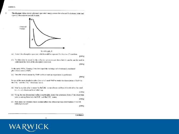
A. Direct dissociation We are familiar by now with “bound” potential energy curves representing the potential energy of a molecule in a particular electronic state (configuration) as a function of internuclear separation: Such curves represent “bonds” arising from bonding orbitals and are stable in the sense that the potential energy of the system is lower than that for isolated atoms / fragments. V R What about the potential energy curves for anti-bonding orbitals?

Dissociative potentials Consider the H 2+ molecule: The 1σ1 , bonding configuration gives rise to a bound potential {X-state} The 2σ1 (or 1σ*1) antibonding configuration gives a purely repulsive Potential Energy potential {A-state} E(1 sσ*) E (1 s) E(1 sσ) H-atom A state {2σ1} σ* σ H-atom X state {1σ1}

Direct dissociation Occurs when a molecule is excited directly to a dissociative potential (or the repulsive wall of a bound potential above its dissociation energy). The absorption is governed by Franck-Condon overlap between the ground state wavefunction and the continuum wavefunctions Characterised by: • Smooth , structureless absorption spectrum • Energetic fragments e. g. , H 2 O A-State, H-X A-state (X=F, Cl, Br) fragments

E. g. , The first absorption band of H 2 O (A ← X) Smooth and featureless! Determined using LIF detection of the OH radical detected

Aside: Continuum Wavefunctions Recall vibrational wavefunctions: As v increases we approach the form of the continuum wavefunction (bound in only one direction) – away from the repulsive wall is the simple sine function of a unrestricted particle.

The Reflection Principle We can understand the smooth featureless absorption spectrum as a reflection of the ground state wavefunction in the excited potential. This is due to the Franck-Condon overlap of the ground-state wavefunction and the continuum functions. λ absorption

Aside: Transition Intensities Governed by the square of the transition dipole moment, μAB: (μ AB ) = 2 [ò ] Ψ B* ˆ μ ΨA dτ 2 where ˆ μ , the dipole moment operator, = å eri i el Applying the Born-Oppenheimer approximation, ΨA = ΨVib ΨA A But ˆ μ only acts on the electronic part so we can write: 2 μ AB = [òΨ *Vib B ] [ò Ψ 2 ΨAVib dτ ] 2 el *el μ Ψ AB A dτ B Franck-Condon Factor: the strength of the transition is dependent on the square of the overlap integral: Good overlap = strong transition

B. Predissociation Excitation to a bound level which is nevertheless coupled to a dissociative state. Degree of predissociation is dependent on the degree of mixing of the two states. This, in turn is dependent on the degree of overlap of the relevant wavefunctions. Overlap: fragments Poor Good Poor

Manifestations: A vibrational level that suffers from predissociation will have a reduced lifetime. Hence in the spectrum of this level the lines will appear diffuse due to lifetime broadening. e. g. , 2+1 REMPI spectrum of jet cooled H 2 O Sharp lines : long lifetimes Diffuse lines due to short lifetimes arising from rapid predissociation

C. Vibrationally mediated photodissociation A EUV Vibrationally mediated photodissociation E OH + H X IR pump (state-selective) RHO----H absorbance F. F. Crim et al. , J. C. P. , 94, 1859 (1991) Leicester, Nov ‘ 04

Strategies in Chemical Physics Traditional: Chemist as a sleuth: Know as much as possible about the “reactants”, allow the reaction to proceed and then characterise the “products” as fully as possible. The science comes in trying to figure out how the system got from one to the other. + Well established methodology (relatively cheap) Intellectually challenging Modern alternative: Chemist as a voyeur: Prepare the reactants and then watch the reaction in real time as it proceeds. + Data relatively simple to interpret More modern sophisticated techniques (£££) required

Watching Reactions Proceed So how fast does a chemical reaction take? It depends what you mean by a reaction: electrons move essentially instantaneously, nuclei much more slowly. So what constitutes making/breaking bonds? A traditional view is that breaking a bond is equivalent to a half collision (i. e. , the two fragments set out as if on a vibration but never come back). Which is how long? Recall classical oscillation frequency: or e. g. , for HCl, a strong single bond; ωe = 2990 cm-1, hence ν = 8. 96 x 1013 Hz (m = 1. 614 x 10 -27 kg, k = 512 Nm-1) Hence the period of vibration is 1/ν = 1. 12 x 10 -14 or 11. 2 fs with atomic motion occurring at speeds of 1 -10 km s-1.

So… …in order to actually “observe” reactions taking place (or at least the nuclear rearrangements which signify the electronic change) we need to be probing on a timescale faster that this. For this reason this area of chemistry is known as “ultrafast” chemistry or “femtochemistry”. Its birth, as with so many advances in this general area was heralded by the invention of ultrafast pulsed lasers. The Nobel Prize in 1999 was awarded to Prof. Ahmed Zewail of Caltech: “For his studies of the transition states of chemical reactions using femtosecond spectroscopy…. for his pioneering investigation of fundamental chemical reactions, using ultra-short laser flashes, on the time scale on which the reactions actually occur. Professor Zewail’s contributions have brought about a revolution in chemistry and adjacent sciences, since this type of investigation allows us to understand predict important reactions. ” To illustrate what is possible in femtochemistry we will study some of the milestone experiments…

Pump-probe experiments All femtochemistry studies comprise “pump-probe” methodologies: A pump pulse (or clocking pulse) at t=0 initiates a change. The system is then monitored by a second, probe pulse and changes detected as a function of time after the pump pulse. • Detection is usually by LIF or REMPI • Close control of time delay of two pulses is performed by moving mirrors: 10 μm path length = 33 fs

1985: Photodissociation of ICN 388 nm 306 nm CN* (A) probe ICN → I-CN* → I + CN (X) pump • Use ~400 fs laser pulses • Detect photons emitted as a function of the pump-probe delay J. Chem. Phys. 89 5141 (1985)

Results I Laser overlap determined by REMPI t From the deconvolution of the two pulses it was inferred that it took around 600 fs to break the bond (or pass through the transition state). Is it possible to measure the transition state itself?

ICN, 1988+ -Transition state spectroscopy As laser pulses got shorter more and more detail began to be revealed… With the probe laser tuned at λ 2 (= 388. 5 nm, on-resonance) the production of CN (x 2 ) is detected via the CN (B ← X) fluorescence. What happens though if the probe wavelength is tuned? Suddenly the experiment is “sensitive to different bond-lengths”.

ICN (cont. ) deconvoluted λ 2= 389. 8 nm 388. 9 nm 390. 4 nm 391. 4 nm

D A C B A B C D

Leads to a very classical picture if we think of wavepackets… The fs laser pulses do not excite individual “stationary states”, ψa, ψb but rather “coherent superpositions” of states: Ψcoh(t) = a(t)ψa + b(t)ψb + c(t)ψc +…. where the coefficients, a(t) are time dependent. Think of the pump pulse creating a “wavepacket” on the excited state which behaves in some senses like a classical particle, i. e. , a localised object in space.

The Na. I system: Probing transition states The potential energy curves: The ground, X-state is ionic in character with a deep minimum and 1/R potential leading to ionic fragments: Na+ + IPE a 1/R R PE Na + I R The first excited state is a weakly bound covalent state with a shallow minimum and atomic fragments.

The non-crossing rule According to Wigner and von Neumann potential energy curves with the same symmetry cannot cross. The best wavefunctions for the system are mixtures of the two curves. At the crossing point the two potentials repel and new adiabatic surfaces result: ionic covalent Na++ INa + I “Avoided crossing” ionic Adiabatic states are mixtures of simple MO or valence bond structures

Behaviour of nuclei at avoided crossings If the nuclei move slowly into the region of an avoided crossing then they will follow the adiabatic path (i. e. , stay on the same adiabatic potential energy surface). If, however , they have enough momentum, the Born-Oppenheimer approximation fails and the system can hop onto the other adiabatic surface effectively ignoring the gap. This is known as non-adiabatic behaviour better modelled using the diabatic curves.

So, the Na. I femtochemistry The wavepacket is launched on the repulsive wall of the excited surface. As it undertakes motion on this surface it encounters the avoided crossing at 6. 93 Ǻ. At this point some molecules will take either path: • Some fragmenting to atomic products • The remainder hopping onto the ionic potential up to the turning point and then coming back down to start all over again.

To visualise: Na++ INa + I The wavepacket continues sloshing about on the excited surface with a small fraction leaking out each time the avoided crossing is encountered left to right.

Probe using LIF: Na* + I Different probe wavelengths, λ 2, probe different internuclear separations as before. I. Probing Na atom products: Steps in the production of Na as more of the wavepacket leaks out each vibration into the Na + I channel. Each step smaller than last (because fewer molecules left) Na++ INa + I

II. Probing [Na—I]* 1 vibrational period a) At the inner turning point: b) c) Signal at t=0 Oscillations as the wavepacket sloshes out of and back into the detection window. d) Peak separation gives the vibrational period (~1200 fs) e) first peak sharpest * * * signals when wavepacket * Large back at inner turning point

Effect of tuning pump wavelength (exciting to different points on excited surface) λpump/nm 300 311 321 339 Different periods indicative of anharmonic potential J. C. P. , 91, 7415, (1989)

At short pump wavelengths few oscillations are seen: λpump/nm Reason: At shorter pump wavelengths the wavepacket is launched from higher on the excited surface and thus the nuclei have more kinetic energy when they encounter the avoided crossing. Hence a larger fraction (nearly all) go straight through the crossing and fall apart into atomic fragments. 300 nm 295 nm 290 nm 284 nm

Tuning λprobe Different probe wavelengths are sensitive to the wavepacket at different internuclear separations. Away from the turning points double peaks appear as the wavepacket passes through in both directions: Detection window ← tim e R→

Chemist as a sleuth: e. g. , High Rydberg time-offlight (photofragment translational spectroscopy) Reading: Ashfold, J. Chem. Phys. 92, 7027, (1990)

A “traditional” form of experiment. . Essentially consists of “reacting” well-characterised reactants, measuring the outcome in terms of the products created, their quantum states and the kinetic energy released and then inferring the likely reactant pathway from the results. Consider the photodissociation reaction: AB → A + B Clearly, from a simple consideration of conservation of energy: Eint, AB + hν → D 0(AB) + Eint, A + Eint, B + KE n. b. , A, B not necessarily atomic fragments

Consider the left hand side, i. e. , reactants: Eint, AB + hν We can clearly control the photon energy used to dissociate the molecule (subject to the energy levels and Franck. Condon factors of the molecule itself). But what about Eint, AB, the internal energy of the molecule? We could “prepare” an individual quantum state spectroscopically. However, it is usual to simply cool the molecule to its lowest quantum state by seeding it within a supersonic expansion (i. e. , within a molecular beam).

. . and the products. . Simply measuring the fragment quantum states will not characterize the dissociation event – we really need correlated fragment distributions and the kinetic energy released simultaneously A (A) + B (X) A (X) + B (A) hν Vibn- rotn levels A (X) + B (X) Different dissociation “channels” How can we identify the different channels?

The key lies in the fact that D 0(AB), Eint, A, Eint, B and the kinetic energy release, are related… Eint, AB + hν → D 0(AB) + Eint, A + Eint, B + KE (1) In the dissociation, momentum must also be conserved. So, in the centre of mass frame: m Av A = m Bv B And KE = ½ m. Av. A 2 + ½ m. Bv. B 2 Not only this but the internal energy of the fragments is encoded in the kinetic energy release according to (1)

Photofragment translational spectroscopy A (A) + B (X) A (X) + B (A) A (X) + B (X) hν Eint, AB Production of each unique fragment quantum states is accompanied by a signature kinetic energy release. Inverted, measurement of the KER identifies the quantum states produced. Due to conservation of momentum it is only necessary to measure the KE of one fragment.

H-atom time of flight The experiment is usually performed with hydrides, looking at the H atom kinetic energy because it, being the lightest fragment, develops most kinetic energy. Detection: Early experiments used direct time of flight ionizing the Hatoms directly. However such schemes suffer from spacecharge effects arising from mutual repulsion of H+ spoiling the kinetic energy resolution. Modern methods use high-n Rydberg states which are highly excited but meta-stable (t > 100 μs) neutral states:

High Rydberg states: Production of H* n ∞ IP 3 Excitation is 2 -stage: 2 Ly-a excites n = 1 → n = 2 13. 6 e. V Ly -a Then another photon from dye laser n = 2 → n > 80 1 Ly-a has energy Ry {1/12 – 1/22} = ¾ x 13. 6 e. V =10. 2 e. V i. e. , λ = 121. 6 nm

Production of Lyman-alpha radiation: 121. 6 nm (82 259 cm-1) is generated by frequency tripling in a gas cell of Kr which has large non-linear susceptibility, χ3 (see lecture 1). 364. 68 nm 121. 6 nm Lens 1 Lens 2 (Li F) Very inefficient process but one of very few ways of generating Ly-a

The experiment is based on neutral atom time of flight: Known flight length, L Photodissociation Laser pulse (t=0) detector H* Atoms are field ionized upon passing through a biased grid directly before detector. H* “Tag” of H-atom fragments resulting (Ly-a + hν)

Measure H*-atom arrival times…. E. g. , for X-H dissociation: Total kinetic energy release = ½ m. Hv. H 2 + ½ m. Xv. X 2 But m Hv H = m X v X Substituting, TKER = ½ m. H{1 + m. H/m. X}v. H 2 But v. H = L / t. H where t. H is the H* arrival time. So measuring the arrival time of just one fragment, the H atom, is enough to determine the channel and the KE release, too.

So. . 0 Eint, HX + hν → jet-cooling Do(HX) + Eint, X + 0 Eint, H + No internal excitation known Unique solutions for each channel TKER measure

e. g. , Ly-a photodissociation of H 2 S 121. 6 nm is so high in energy that several channels are open: H 2 S + 121. 6 nm → → (→ (→ (→ H + SH (X 2Π) H + SH (A 2Σ) H + S (3 P) H + S (1 D) H 2 + S (3 P) H 2 + S (1 D) H 2 + S (1 S) KE < 6. 3 e. V KE < 2. 5 e. V KE < 2. 6 e. V KE < 1. 4 e. V KE < 7. 1 e. V ) KE < 5. 9 e. V) KE < 4. 3 e. V) H-atom TOF (or High Rydberg time of flight HRTOF) is only sensitive to the first 4 channels since the others would not liberate H atoms.

Results: 121. 6 nm photolysis of H 2 S Time, t. H /μs Each peak corresponds to fragmentation into a different rovibronic channel. TKER / e. V Ashfold et al. , J. Chem. Phys. , 92, 7027, (1990)

Results: 121. 6 nm photolysis of H 2 S Alternative fragmentation channels: Main channel Almost no ground state products

Major Results: Primary fragment channels are: H + SH (A 2Σ) H + S (1 D) By fitting the SH rovibrational structure we can deduce: • Most A- state SH is formed in v=0 with rotational excitation extending all the way to the dissociation limit. • Evidence of small vibrational excitation up to v=4, allowing accurate determination of ωe and ωexe for A-state if not already known. • Generation of SH (X 2Π) represents a very minor channel • H + SH (A 2Σ) total kinetic energy determined to be 2. 47 e. V • Added to the known SH X-A spacing this yields an H 2 S ground state dissociation energy of 3. 903 0. 005 e. V (very precise and accurate)

Which tells us what? Ground state H 2 S + hν yields an excited 1 A 1 state (by selection rules) – the B-state There are 3 possible fragmentation pathways: • Transfer to H 2 S X-state dissociation continuum via conical intersection (non-adiabatic) – would yield ground state products. • Transfer to the dissociative H 2 S A-state via the linear H-SH geometry which would also yield ground state fragments • Dissociation on the B-state surface –yielding SH (A) + H Clearly the third dominates the dissociation dynamics.

Comparison with H 2 O dynamics H 2 O Combination of OH (X) in high rot. states and some OH (A) H 2 S

H 2 O / H 2 S comparison H 2 O H 2 S Dominant products 90% OH (X) state 10% OH (A) state Almost all SH (A) state Some H + S Vibrational / rotational distributions Both X and A state fragments formed vibrationally cold. High rotational excitation Mainly SH A(v=0) with large rot excitation (up to D 0) Some higher v with lower rot excitation Implied dominant Most fragmentation Primary fragmentation takes mechanism follows from crossing place on the excited Bonto the X surface state surface without via a conical surface hopping. intersection i. e. , significant differences from seemingly similar systems

CH 405 part I Conclusions Hopefully this module has give you an insight into the some of the technologies and methodologies used in modern Chemical Physics. It goes without saying that we have hardly touched the surface but maybe you can now appreciate the level of detail it is possible to extract from these sophisticated experiments. This is a difficult module to assess – all I can do is recommend that you do as many past papers as possible and the model questions attached. These will form the basis for an examples class in Week 20.

CH 405 part I: Example Questions 1) Answer both parts: a) In terms of a single photon and a two level system, explain the different ways in which light can interact with matter. Explain what is meant by population inversion and why it is a necessary condition for laser action. How is this population inversion effected in the gas phase Helium-Neon laser? What properties of laser radiation distinguish it from light produced by other means? [50%] b) In a High Rydberg Time of Flight (HRTOF) experiment, an Ar. F (193 nm) excimer laser is used to photodissociate jet-cooled water in its first absorption band. The fastest H atom produced had a kinetic energy of 10870 cm-1. Calculate the dissociation energy of water. [50%]

2) Describe one method with which it is possible determine the quantum state distribution of a sample of gaseous molecules. [30%] What factors contribute to the width of spectral lines? [20%] Explain the following: i) In absorption the spectrum of water in the region 130 – 190 nm is smooth and featureless. ii) 248 nm light is not absorbed by gaseous water molecules. The same light is however absorbed if the water molecules are subjected to an intense infra-red laser just before the 248 nm light pulse. iii) The OH A 2 (v=0) - X 2Π(v=0) band is observed in LIF as a series of sharp peaks whilst the OH A 2 (v=1) - X 2Π(v=0) band consists of much more diffuse peaks. [50]

3) Zewail has pioneered the technique of femtochemistry by which it is possible to follow simple chemical reactions in real time. The most famous example is his study of the Na. I system. a) Draw the potential energy curves involved in this system and account for the difference in their form. [25] b) Explain briefly how the experiment is performed including the detection method used and how it can be used to differentiate different bond lengths. c) d) [40] Sketch the form of the results obtained indicating the type of information obtained from them. [35] You should also attempt the exam questions from 2000 – 2007 inclusive.