Ch 4 Time Response 4 2 Poles Zeros

 = N(s)/D(s)")
 = (s+2)/(s+5)")
 C(t) =")

")
 = Cf(t) + Cn(t) = 1 - e-at to a unit step Figure")
 C(t) = 1 -")
 暫態反應參數: time constant =")
 =")


 = K 1")
 =")
 = Cf(t) + Cn(t) 3. Undamped responses two imaginary poles: ±")
 = Cf(t) + Cn(t) 4. Critically damped responses two real poles:")
=? H. W. skill-assessment exercise")


 → Poles → ωn = S")


 與")
 H. W. 證明 Inverse Laplace C(s) (4. 27) → C(t) (4. 28)")
/ Cfinal� × 100% Ts:系統進入 ± 2%")
 →")
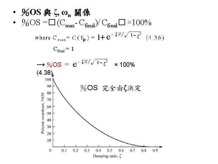
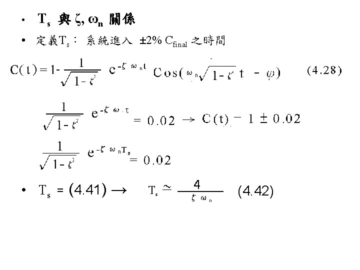
 Figure 4. 16 Normalized rise time")


, system T 2(s), and system")

/(-b + c)")
 Step response of a nonminimum-phase system")
 Explain (4. 86) & (4. 87); Why (4. 87)")
- Slides: 64
Ch. 4 Time Response
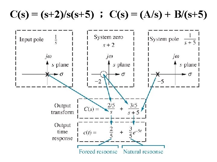
4. 2 Poles, Zeros, and System Response • T. F. = G(s) = N(s)/D(s) • Poles S之值→G(s)= ∞ or D(s)=0 • Zeros S之值→ G(s)= 0 or N(s)=0 • Fig. 4. 1 C(s) = (s+2)/s(s+5) 說明poles and zeros
4. 2 Poles, Zeros, and System Response • T. F. = G(s) = (s+2)/(s+5) • Fig. 4. 1 C(s) = (s+2)/s(s+5) C(s) = (A/s)+B/(s+5) = (As+5 A+Bs)/s(s+5) C(t)=Cf(t)+Cn(t) pole 越左 系統反應越快 zero 影響系統振幅
Figure 4. 2 Effect of a realaxis pole upon transient response (暫態反應) C(t) = Cforced(t) + Cnatural(t) = 1 - e-at to a unit step input Example 4. 1 Figure 4. 3 p. 165 or ? 求 C(t) = ? 自修
Part 2
4. 3 First-Order Systems Figure 4. 4 a. First-order system; b. pole plot C(s) = a/s(s+a) C(t) = Cforced(t) + Cnatural(t) = 1 - e-at R(s) = 1/s
C(t) = Cf(t) + Cn(t) = 1 - e-at to a unit step Figure 4. 5 First-order system response to a unit step 系統反應由time constant (1/a)完全 決定 (i. e. 系統規 格)
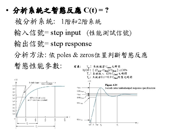
Figure 4. 5 系統反應由time constant完全決 定 (i. e. 系統規格 ) C(t) = 1 - e-at r(t)=1 定義暫態反應參數: time constant rise time settling time
Figure 4. 5 系統反應由time constant完全決 定 (i. e. 系統規格 ) 暫態反應參數: time constant = 1/a = 1/exponential frequency C(t) = 0 → 0. 63 C(t) = 1 - e-at = 0. 63 → t = 1/a (C(t) = 1 - e-1 = 1 -0. 37 = 0. 63) rise time = Tr = (2. 31/a)-(0. 11/a) = 2. 2/a (eq. 4. 9) C(t) = 0. 1 → 0. 9 Tr = t 0. 9–t 0. 1 (C(t 0. 9) = 0. 9; C(t 0. 1) = 0. 1) settling time = Ts = 4/a i. e. C(Ts)=0. 98 (eq. 4. 10)
Figure 4. 6 Laboratory results of a system step response test 求證 G(s) = 5. 54/(s+7. 7) HW skill-assessment exercise 4. 2
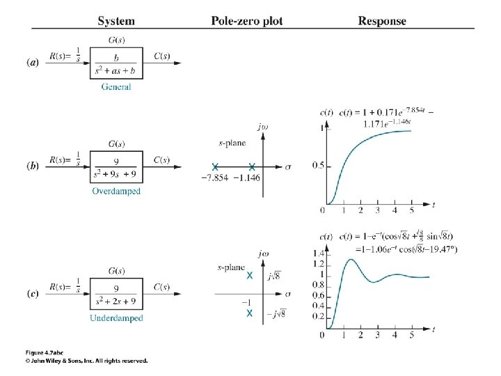
4. 4 Second-Order Systems: Introduction Figure 4. 7 Second-order systems, pole plots, and step responses
Figure 4. 8 Second-order step response components generated by complex poles e-t 配合Fig. 4. 7(c)說明 underdamped system C(t) = 1 -1. 06 e-t Cos(2. 598 t-19. 47 o)
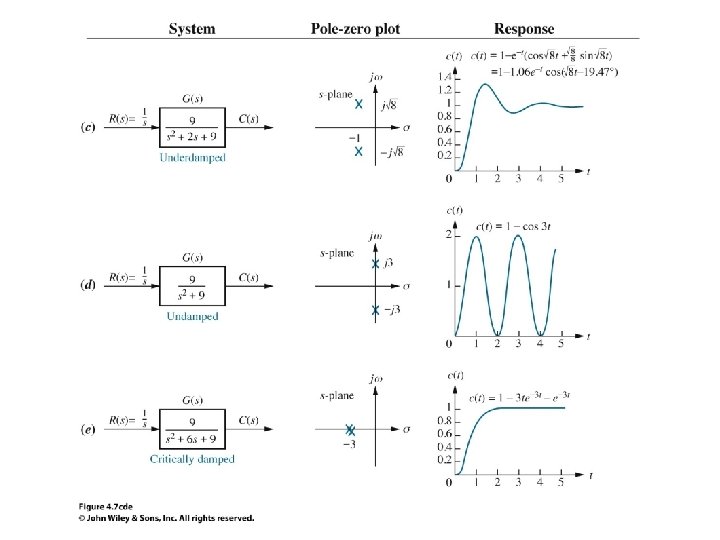
Figure 4. 10 Step responses for second-order system damping cases
Part 3
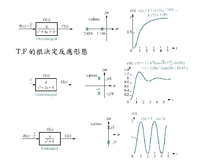
Natural responses: 1. Overdamped responses two real poles: -σ1, -σ2 Cn(t) = K 1 e- σ1 t + K 2 e- σ2 t C(t) =1+ K 1 e- σ1 t + K 2 e- σ2 t C(t) = Cf(t) + Cn(t)
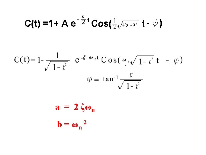
Natural responses: 2. Underdamped responses two complex poles: -σd ± j ωd Cn(t) = A e- σd t Cos(ωdt - ψ) C(t) =1+ A e- σd t Cos(ωdt - ψ) C(t) = Cf(t) + Cn(t)
Natural responses: C(t) = Cf(t) + Cn(t) 3. Undamped responses two imaginary poles: ± j ω1 Cn(t) = A Cos(ω1 t - ψ) C(t) =1+ A Cos(ω1 t - ψ)
Natural responses: C(t) = Cf(t) + Cn(t) 4. Critically damped responses two real poles: -σ1, -σ1 Cn(t) = K 1 e- σ1 t + K 2 t e- σ1 t C(t) =1+ K 1 e- σ1 t + K 2 t e- σ1 t
Figure 4. 9 System for Example 4. 2 Find C(t)=? H. W. skill-assessment exercise 4. 3
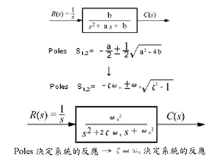
4. 5 The General Second-Order System • 1階系統之反應由 time constant 決定 2階系統之反應由 ωn and ζ決定 • Natural frequency ωn ωn≡ frequency of oscillation when system damping set to zero • Damping ratio ζ (Zeta) ζ≡ exponential decay frequency / natural frequency ≡ σ1 / ωn
Poles S 1, 2 =
Poles 1. With damping neglected (i. e. a=0) → Poles → ωn = S 1, 2 = ± j S 1, 2 = 不消耗能量系統 =± jωn → ωn 2 = b
Poles S 1, 2 = 2. Defining damping ratio (ζ≡ exponential decay frequency / natural frequency) → a = 2 ζωn Poles S 1, 2 =
S 1, 2 = ζ值 決定sys response 之類別 i. e. 決定系統特性 ωn 決定振動頻率 Figure 4. 11 Second-order response as a function of damping ratio
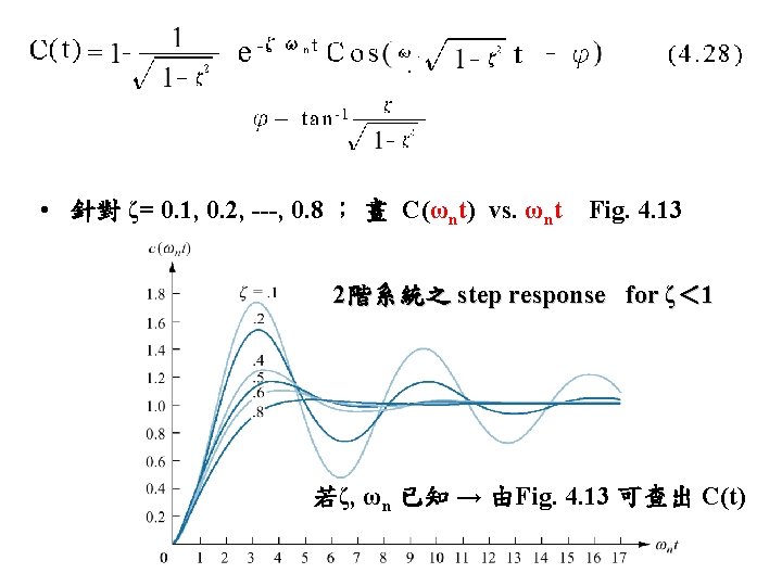
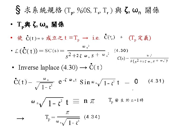
4. 6 Underdamped Second-Order Systems • 目標: 定義系統規格 (Tp, %OS, Ts, Tr ) 與 ζ, ωn 關係 • 求2階系統之 step response for ζ< 1 通分 由係數比較 求K 1 , K 2 , K 3 Inverse Laplace C(s) (4. 27) i. e. underdamped system → (4. 27) p. 177 → C(t) (4. 28)
(4. 27) H. W. 證明 Inverse Laplace C(s) (4. 27) → C(t) (4. 28)
定義: Tp: 系統抵達 Cmax 之時間 %OS:� (Cmax- Cfinal)/ Cfinal� × 100% Ts:系統進入 ± 2% Cfinal 之時間 Tr:系統由 0. 1→ 0. 9 Cfinal所需之時間 Figure 4. 14 Second-order underdamped response specifications
證明 H. W. • Inverse laplace (4. 30) →
• Tr 與 ζ, ωn 關係 (無法導出公式) Figure 4. 16 Normalized rise time vs. damping ratio for a second-order underdamped response
• Ex. 4. 5 self study p. 196 • 由 pole 在 s-plane 之位置找 ζ, ωn Poles S 1, 2 = ωd:damped frequency of oscillation ζωn=σd exponential decay frequency ζ= cosθ
說明 H. W. Poles S 1, 2 = ωd:damped frequency of oscillation ζωn=σd exponential decay frequency ζ= cosθ
• Tp= constant;Constant peak time; ωd = constant • Ts= constant;Constant settling time; σd = constant • ζ= constant;Constant %OS; θ = constant ζ= cosθ Figure 4. 18 Lines of constant Tp , Ts , and %OS
Figure 4. 19 Step responses of second-order underdamped systems as poles move: a. with constant real part; b. with constant imaginary part; c. with constant damping ratio
Ex. 4. 6 Self study Find ζ; ωn ; %OS ;Ts; Tp • H. W. Skill-Assessment Excises 4. 5 p. 186 Given T. F. G(s) Find ζ; ωn ; %OS ;Ts; Tp ; Tr
Example 4. 7 Figure 4. 21 1/2 It’s about system design. System specs. : 欲 Ts= 2 sec. , %OS= 20% 求 J=? D=? where input torque T(t) =step input 想要的系統反應→想要的pole位置→ G(s)設計 i. e. G(s)參數設計, 亦稱系統設計 i. e. 找 ζ; ωn
Example 4. 7 ωn 2 = K/J 2/2 2ζωn= 4 = D/J Ts= 2 找 ζ; ωn 2ζωn= 4 %OS= 20% →ζ= 0. 456 → ωn = 0. 052 → K/J = 0. 052 D/J = 4 If K = 5 N-m/rad → J=0. 26 kg-m 2 D=1. 04 N-m-S/rad
4. 7 System Response with Additional Poles Figure 4. 23 three-pole system: a. pole plot; b. nondominant pole is near dominant second-order pair (Case I), far from the pair (Case II), and at infinity (Case III) 重點: dominant second-order pair
• 重點: dominant second-order pair 數學證明1 e. g. 1 3階 system: • step response C(s) = (4. 57) p. 202 If system represented by its dominant second-order pair of poles
• 重點: dominant second-order pair 數學證明2 e. g. 2 3階 system: • nondominant pole =- c A=1 ca) B=(ca-c 2)/(c 2+b-ca) C=(ca 2 -c 2 a-bc)/(c 2+b-ca) D =-b/(c 2+b- 當 c→∞ D=0 i. e. nondominant pole 對系統無影響
Figure 4. 24 Step responses of system T 1(s), system T 2(s), and system T 3(s) (eq. 4. 62 - 4. 64) T 1(s): 2階; T 2(s): 3 rd pole at -10; T 3(s): 3 rd pole at -3 • Additional pole (1) slow the response (2) reduce the peak
H. W. Skill-Assessment Exercise 4. 6 p. 190
4. 8 System Response with Zeros system A = (-b + a)/(-b + c) B = (-c + a)/(-c + b) 經通分及係數比對 當 a >> b , c Figure 4. 25 Effect of adding a zero to a two-pole system where zero at LHP 1. Zero 改變系統反應之shape不大 2. Zero 增加 peak value Zero looks like a simple gain factor (4. 69) Two poles at -1 ± j 2, 828
Figure 4. 26 (zero at RHP) Step response of a nonminimum-phase system
Ex. 4. 10 (pole-zero cancellation) Explain (4. 86) & (4. 87); Why (4. 87) 可進行 pole-zero cancellation? → (4. 89) H. W. Skill-Assessment Exercise 4. 7 p. 195 用Excel畫系統反應 驗證是否可執行pole-zero cancellation?