Ch 4 Discrete Probability Distributions Sections 4 1
Ch. 4 – Discrete Probability Distributions Sections 4. 1, 4. 2, and 4. 3
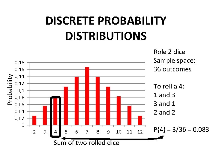
Probability DISCRETE PROBABILITY DISTRIBUTIONS 0, 18 0, 16 0, 14 0, 12 0, 1 0, 08 0, 06 0, 04 0, 02 0 Role 2 dice Sample space: 36 outcomes To roll a 4: 1 and 3 3 and 1 2 and 2 2 3 4 5 6 7 8 9 10 11 12 Sum of two rolled dice P{4} = 3/36 = 0. 083
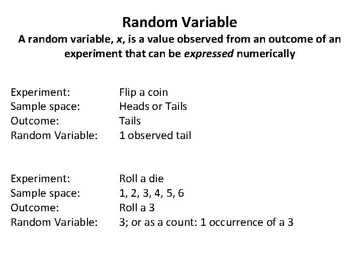
Random Variable A random variable, x, is a value observed from an outcome of an experiment that can be expressed numerically Experiment: Sample space: Outcome: Random Variable: Flip a coin Heads or Tails 1 observed tail Experiment: Sample space: Outcome: Random Variable: Roll a die 1, 2, 3, 4, 5, 6 Roll a 3 3; or as a count: 1 occurrence of a 3
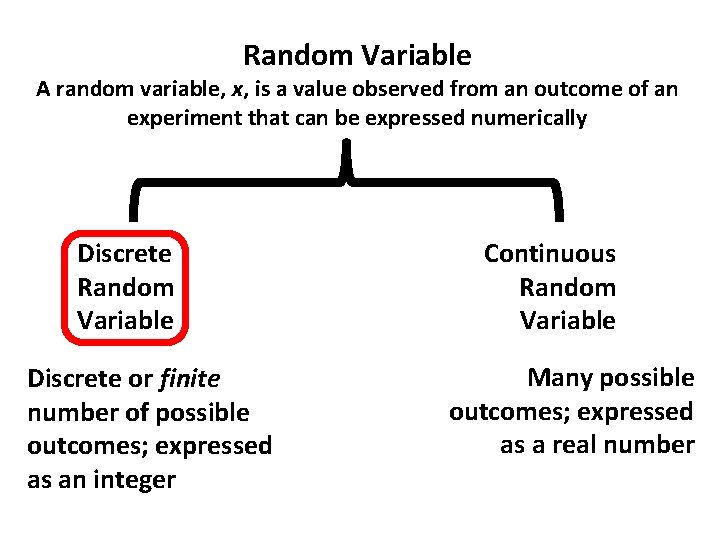
Random Variable A random variable, x, is a value observed from an outcome of an experiment that can be expressed numerically Discrete Random Variable Discrete or finite number of possible outcomes; expressed as an integer Continuous Random Variable Many possible outcomes; expressed as a real number
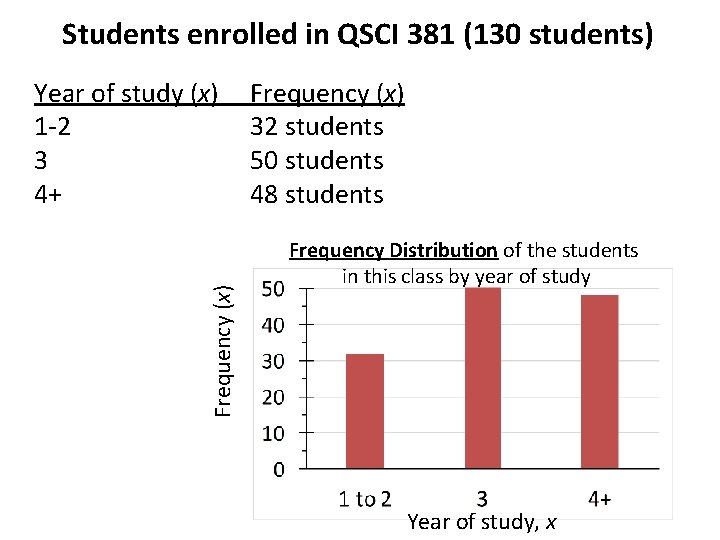
Students enrolled in QSCI 381 (130 students) Frequency (x) Year of study (x) 1 -2 3 4+ Frequency (x) 32 students 50 students 48 students Frequency Distribution of the students in this class by year of study Year of study, x
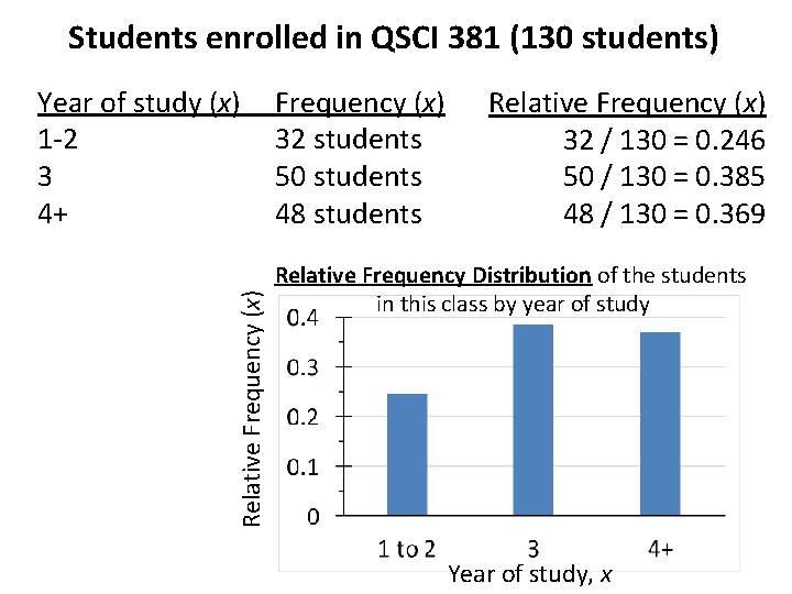
Students enrolled in QSCI 381 (130 students) Relative Frequency (x) Year of study (x) 1 -2 3 4+ Frequency (x) 32 students 50 students 48 students Relative Frequency (x) 32 / 130 = 0. 246 50 / 130 = 0. 385 48 / 130 = 0. 369 Relative Frequency Distribution of the students in this class by year of study Year of study, x
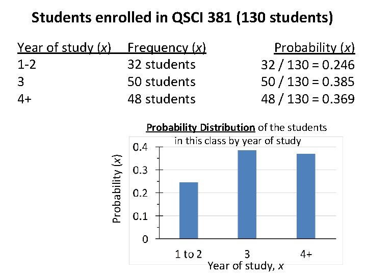
Students enrolled in QSCI 381 (130 students) Year of study (x) 1 -2 3 4+ Frequency (x) 32 students 50 students 48 students Probability (x) 32 / 130 = 0. 246 50 / 130 = 0. 385 48 / 130 = 0. 369 Probability (x) Probability Distribution of the students in this class by year of study Year of study, x
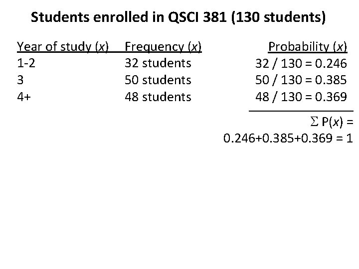
Students enrolled in QSCI 381 (130 students) Year of study (x) 1 -2 3 4+ Frequency (x) 32 students 50 students 48 students Probability (x) 32 / 130 = 0. 246 50 / 130 = 0. 385 48 / 130 = 0. 369 ________ S P(x) = 0. 246+0. 385+0. 369 = 1
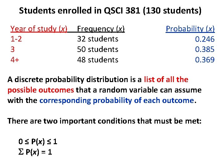
Students enrolled in QSCI 381 (130 students) Year of study (x) 1 -2 3 4+ Frequency (x) 32 students 50 students 48 students Probability (x) 0. 246 0. 385 0. 369 A discrete probability distribution is a list of all the possible outcomes that a random variable can assume with the corresponding probability of each outcome. There are two important conditions that must be met: 0 ≤ P(x) ≤ 1 S P(x) = 1
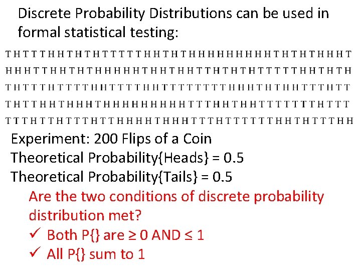
Discrete Probability Distributions can be used in formal statistical testing: Experiment: 200 Flips of a Coin Theoretical Probability{Heads} = 0. 5 Theoretical Probability{Tails} = 0. 5 Are the two conditions of discrete probability distribution met? ü Both P{} are ≥ 0 AND ≤ 1 ü All P{} sum to 1
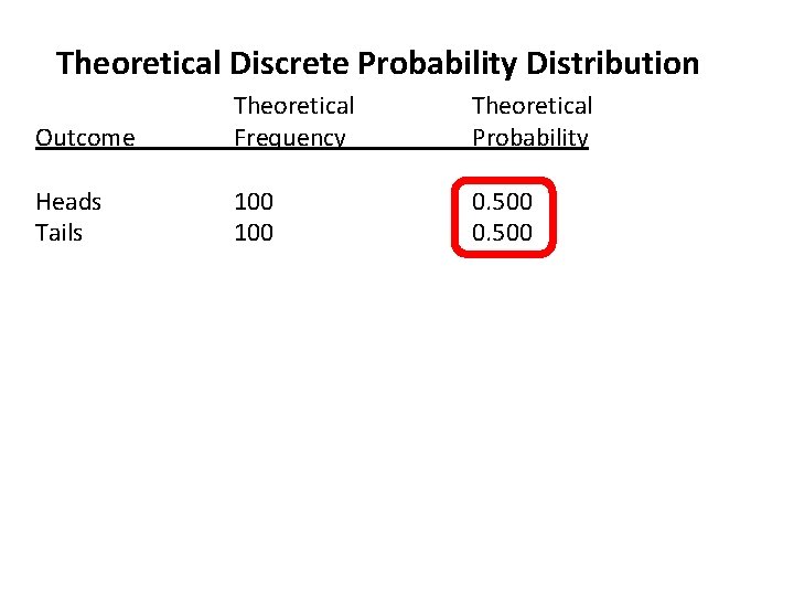
Theoretical Discrete Probability Distribution Outcome Theoretical Frequency Theoretical Probability Heads Tails 100 0. 500 Experimental Discrete Probability Distribution Outcome Observed Frequency Observed Probability Heads Tails 97 103 0. 485 0. 515
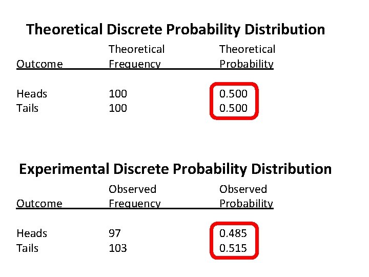
Theoretical Discrete Probability Distribution Outcome Theoretical Frequency Theoretical Probability Heads Tails 100 0. 500 Experimental Discrete Probability Distribution Outcome Observed Frequency Observed Probability Heads Tails 97 103 0. 485 0. 515
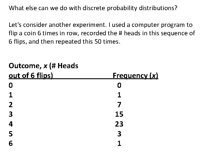
What else can we do with discrete probability distributions? Let's consider another experiment. I used a computer program to flip a coin 6 times in row, recorded the # heads in this sequence of 6 flips, and then repeated this 50 times. Outcome, x (# Heads out of 6 flips) 0 1 2 3 4 5 6 Frequency (x) 0 1 7 15 23 3 1
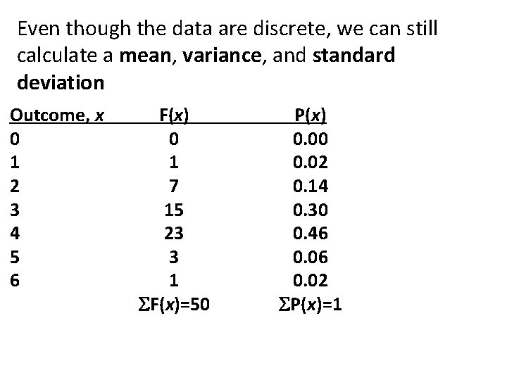
Even though the data are discrete, we can still calculate a mean, variance, and standard deviation Outcome, x 0 1 2 3 4 5 6 F(x) 0 1 7 15 23 3 1 SF(x)=50 P(x) 0. 00 0. 02 0. 14 0. 30 0. 46 0. 02 SP(x)=1

The mean from a discrete probability distribution is based on the mean of the discrete random variables = m = Sx. P(x)= Expected Value of x = E(x) Outcome, x 0 1 2 3 4 5 6 F(x) 0 1 7 15 23 3 1 SF(x)=50 P(x) 0. 00 0. 02 0. 14 0. 30 0. 46 0. 02 SP(x)=1
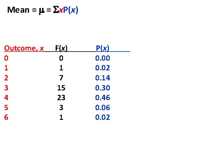
Mean = m = Sx. P(x) Outcome, x 0 1 2 3 4 5 6 F(x) 0 1 7 15 23 3 1 P(x) 0. 00 0. 02 0. 14 0. 30 0. 46 0. 02 x. P(x) 0 × 0. 00 = 0. 00 1 × 0. 00 = 0. 00 2 × 0. 00 = 0. 24 3 × 0. 00 = 0. 99 4 × 0. 00 = 1. 88 5 × 0. 00 = 0. 35 6 × 0. 00 = 0. 12 Sx. P(x) = 3. 6
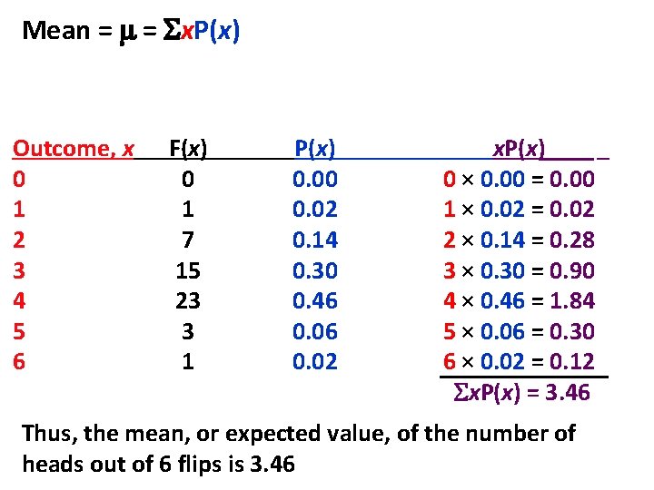
Mean = m = Sx. P(x) Outcome, x 0 1 2 3 4 5 6 F(x) 0 1 7 15 23 3 1 P(x) 0. 00 0. 02 0. 14 0. 30 0. 46 0. 02 x. P(x) 0 × 0. 00 = 0. 00 1 × 0. 02 = 0. 02 2 × 0. 14 = 0. 28 3 × 0. 30 = 0. 90 4 × 0. 46 = 1. 84 5 × 0. 06 = 0. 30 6 × 0. 02 = 0. 12 Sx. P(x) = 3. 46 Thus, the mean, or expected value, of the number of heads out of 6 flips is 3. 46
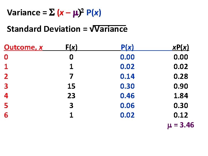
Variance = S (x – m)2 P(x) Standard Deviation = √Variance Outcome, x 0 1 2 3 4 5 6 F(x) 0 1 7 15 23 3 1 P(x) 0. 00 0. 02 0. 14 0. 30 0. 46 0. 02 x. P(x) 0. 00 0. 02 0. 28 0. 90 1. 84 0. 30 0. 12 m = 3. 46
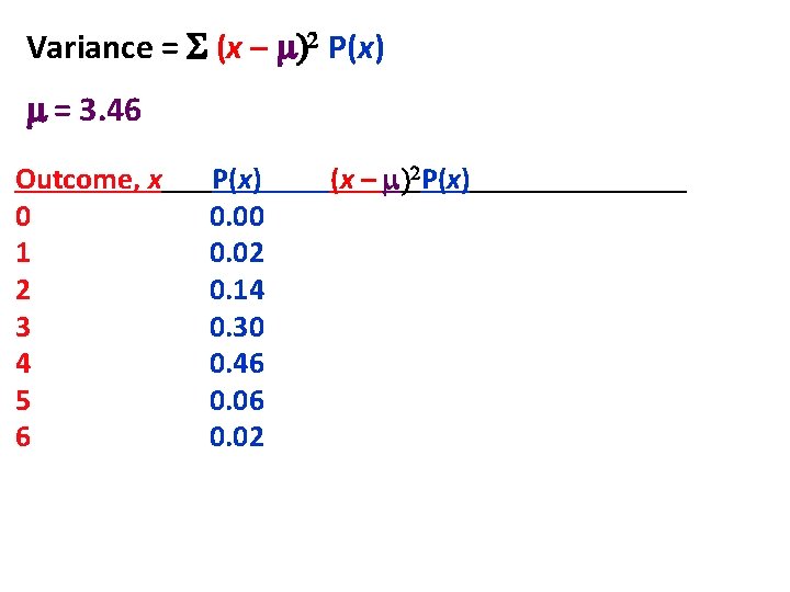
Variance = S (x – m)2 P(x) m = 3. 46 Outcome, x 0 1 2 3 4 5 6 P(x) 0. 00 0. 02 0. 14 0. 30 0. 46 0. 02 (x – m)2 P(x) (0– 3. 6)2 × 0. 00 (1– 3. 6)2 × 0. 00 (2– 3. 6)2 × 0. 12 (3– 3. 6)2× 0. 33 (4– 3. 6)2× 0. 47 (5– 3. 6)2× 0. 07 (6– 3. 6)2× 0. 02 = 0. 00 = 0. 31 = 0. 12 = 0. 08 = 0. 14 = 0. 12
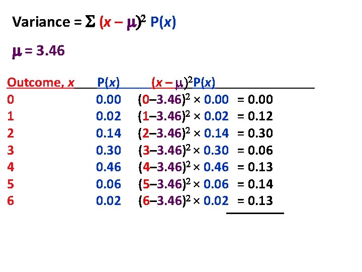
Variance = S (x – m)2 P(x) m = 3. 46 Outcome, x 0 1 2 3 4 5 6 P(x) 0. 00 0. 02 0. 14 0. 30 0. 46 0. 02 (x – m)2 P(x) (0– 3. 46)2 × 0. 00 (1– 3. 46)2 × 0. 02 (2– 3. 46)2 × 0. 14 (3– 3. 46)2 × 0. 30 (4– 3. 46)2 × 0. 46 (5– 3. 46)2 × 0. 06 (6– 3. 46)2 × 0. 02 = 0. 00 = 0. 12 = 0. 30 = 0. 06 = 0. 13 = 0. 14 = 0. 13
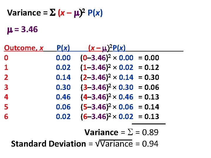
Variance = S (x – m)2 P(x) m = 3. 46 Outcome, x 0 1 2 3 4 5 6 P(x) 0. 00 0. 02 0. 14 0. 30 0. 46 0. 02 (x – m)2 P(x) (0– 3. 46)2 × 0. 00 (1– 3. 46)2 × 0. 02 (2– 3. 46)2 × 0. 14 (3– 3. 46)2 × 0. 30 (4– 3. 46)2 × 0. 46 (5– 3. 46)2 × 0. 06 (6– 3. 46)2 × 0. 02 = 0. 00 = 0. 12 = 0. 30 = 0. 06 = 0. 13 = 0. 14 = 0. 13 Variance = S = 0. 89 Standard Deviation = √Variance = 0. 94
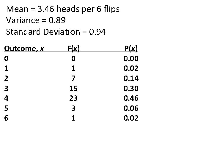
Mean = 3. 46 heads per 6 flips Variance = 0. 89 Standard Deviation = 0. 94 Outcome, x 0 1 2 3 4 5 6 F(x) 0 1 7 15 23 3 1 P(x) 0. 00 0. 02 0. 14 0. 30 0. 46 0. 02
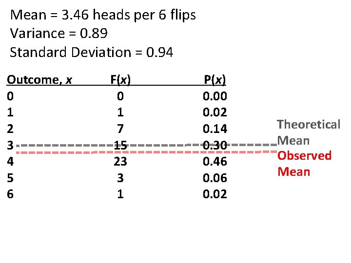
Mean = 3. 46 heads per 6 flips Variance = 0. 89 Standard Deviation = 0. 94 Outcome, x 0 1 2 3 4 5 6 F(x) 0 1 7 15 23 3 1 P(x) 0. 00 0. 02 0. 14 0. 30 0. 46 0. 02 Theoretical Mean Observed Mean
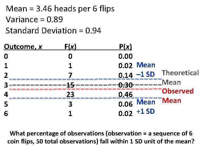
Mean = 3. 46 heads per 6 flips Variance = 0. 89 Standard Deviation = 0. 94 Outcome, x 0 1 2 3 4 5 6 F(x) 0 1 7 15 23 3 1 P(x) 0. 00 0. 02 0. 14 0. 30 0. 46 0. 02 Mean – 1 SD Theoretical Mean Observed Mean +1 SD What percentage of observations (observation = a sequence of 6 coin flips, 50 total observations) fall within 1 SD unit of the mean?
- Slides: 24