Ch 2 The Normal Distribution 2 1 Density

Ch 2 The Normal Distribution 2. 1 Density Curves and the Normal Distribution 2. 2 Standard Normal Calculations

• We have a clear strategy for exploring data on a single quantitative variable – Plot Data, usually Histogram or Stemplot – Calculate numerical summaries – Describe the CUSS • New step: – If the overall pattern is very regular (not necessarily symmetric), we can describe it with a smooth curve

Density Curves • Easier to work with a smooth curve than with a histogram • The curve describes what proportions of the observations fall within each range of values • Total area under the curve is exactly 1 • Always on or above the horizontal axis

Density Curves The shaded area is the proportion of observations taking values between 7 and 8

Median and Mean of Density Curve • Median – Equal-Areas Point. Half the area to its left and half its area to its right – Quartiles divide area into quarters • Mean – Balance point at which the curve would balance if it were made of solid material – Pulled towards skewing

At which of these points on each curve do the mean and median fall? Median: B Median: A Median: B Mean: C Mean: A

New Notation • Density Curve is an idealized description of data. Must distinguish between mean and standard deviation of a density curve versus those of actual observations • Actual Observations: • Idealized distributions:

Normal Distributions • Normal Distributions: – Symmetric, Single-Peaked, Bell-Shaped – Always described by giving

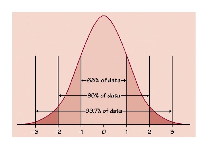
“Empirical” or “ 68 -95 -99. 7” Rule For any normal distribution: • 68% of the observations fall within 1 standard deviation of the mean • 95% of the observations fall within 2 standard deviations of the mean • 99. 7% of the observations fall within 3 standard deviations of the mean

• 2. 6 MEN’S HEIGHTS The distribution of heights of adult American men is approximately normal with mean 69 inches and standard deviation 2. 5 inches. Draw a normal curve on which this mean and standard deviation are correctly located.

2. 2 Standard Normal Calculations • We can “standardize” all normal distributions by measuring in units of size about the mean • Standardizing Observations If x is an observation from a distribution that has mean and standard deviation , then standardized value of x is Called z-score. The z-score tells us how many standard deviations the original observation falls from the mean and in which direction
")
Standard Normal Distribution N(1, 0)
 • Ex: Find the proportion of observations from the")
Standard Normal Table (Table A) • Ex: Find the proportion of observations from the standard normal table that are less than 2. 22 0. 9868

• Ex: The heights of young women are approximately normal N(64. 5”, 2. 5”). Find the standardized height of a woman who is 68” tall.

• What proportion of women are less than 68” tall? About 0. 9192 or 91. 92% of women are less than 68” tall.
. Levels above")
• Ex: Cholesterol Level for 14 year old boys N(170, 30). Levels above 240 may require medical attention. Units: cholesterol per deciliter of blood. – What % of 14 yr. old boys have more than 240 mg/dl cholesterol?

• Looking for proportions of values above 2. 33. • Table A gives proportions below a z score. Can we still use the table to answer the question? Proportion of 14 yr. old boys with a cholesterol level greater than 240 is approx. . 0099 or. 99%

• What proportion of 14 yr old boys have blood cholesterol between 170 and 240 mg/dl? • Looking for: • Standardize both scores: The proportion of boys have blood cholesterol between 170 and 240 is 0. 4901 or about 49%
. To earn in")
• EX: Scores on the SAT Verbal follow N(505, 110). To earn in the top 10% how high must a student score? Closest to 0. 9 is 0. 8997 which corresponds to z=1. 28 x = 646…. does this make sense in the context of the problem?

Assessing Normality • Construct a histogram or stem-plot to verify bell shape • Calculate the percent of observations within 1 and 2 standard deviations from the mean and compare to empirical rule • Construct a normal probability plot using your calculator. If data is close to normal, plotted points will lie in close to a straight line.

2. 26 CAVENDISH AND THE DENSITY OF THE EARTH Repeated careful measurements of the same physical quantity often have a distribution that is close to normal. Here are Henry Cavendish’s 29 measurements of the density of the earth, made in 1798. (The data give the density of the earth as a multiple of the density of water. ) 5. 50 5. 61 4. 88 5. 07 5. 26 5. 55 5. 36 5. 29 5. 58 5. 65 5. 57 5. 53 5. 62 5. 29 5. 44 5. 34 5. 79 5. 10 5. 27 5. 39 5. 42 5. 47 5. 63 5. 34 5. 46 5. 30 5. 75 5. 68 5. 85 (a) Construct a stemplot to show that the data are reasonably symmetric. (b) Now check how closely they follow the 68– 95– 99. 7 rule. Find and s, then count the number of observations that fall between – s and s, between – 2 s and 2 s, and between – 3 s and 3 s. Compare the percents of the 29 observations in each of these intervals with the 68– 95– 99. 7 rule. (c) Use your calculator to construct a normal probability plot
- Slides: 22