Ch 2 Linear Discriminants Stephen Marsland Machine Learning
![Incremental Stochastic Gradient Descent • Batch mode : gradient descent w=w - ED[w] over Incremental Stochastic Gradient Descent • Batch mode : gradient descent w=w - ED[w] over](https://slidetodoc.com/presentation_image/4d6ab29cdec775acee6d7b5bb0440b94/image-33.jpg)
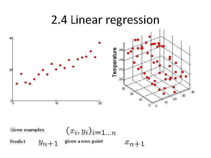
![Ordinary Least Squares [summary] Given examples Let For example Let n d Minimize Predict Ordinary Least Squares [summary] Given examples Let For example Let n d Minimize Predict](https://slidetodoc.com/presentation_image/4d6ab29cdec775acee6d7b5bb0440b94/image-45.jpg)
- Slides: 54

Ch. 2: Linear Discriminants Stephen Marsland, Machine Learning: An Algorithmic Perspective. CRC 2009 based on slides from Stephen Marsland, from Romain Thibaux (regression slides), and Moshe Sipper Longin Jan Latecki Temple University latecki@temple. edu

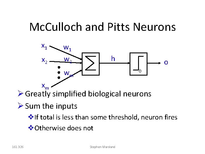
Mc. Culloch and Pitts Neurons x 1 x 2 w 1 w 2 h wm o xm Greatly simplified biological neurons Sum the inputs If total is less than some threshold, neuron fires Otherwise does not 161. 326 Stephen Marsland

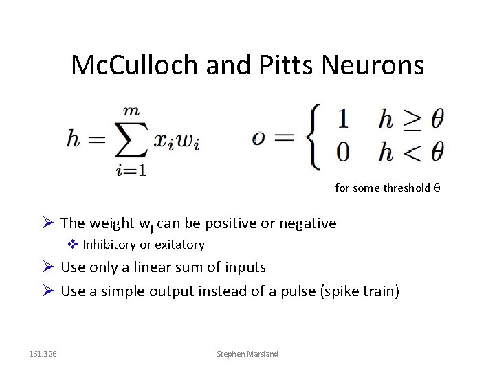
Mc. Culloch and Pitts Neurons for some threshold The weight wj can be positive or negative Inhibitory or exitatory Use only a linear sum of inputs Use a simple output instead of a pulse (spike train) 161. 326 Stephen Marsland

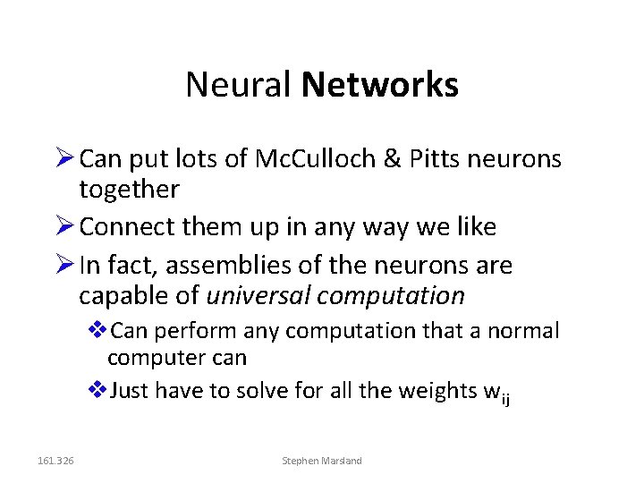
Neural Networks Can put lots of Mc. Culloch & Pitts neurons together Connect them up in any way we like In fact, assemblies of the neurons are capable of universal computation Can perform any computation that a normal computer can Just have to solve for all the weights wij 161. 326 Stephen Marsland

Training Neurons Adapting the weights is learning How does the network know it is right? How do we adapt the weights to make the network right more often? Training set with target outputs Learning rule 161. 326 Stephen Marsland

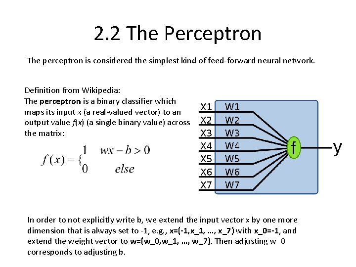
2. 2 The Perceptron The perceptron is considered the simplest kind of feed-forward neural network. Definition from Wikipedia: The perceptron is a binary classifier which maps its input x (a real-valued vector) to an output value f(x) (a single binary value) across the matrix: In order to not explicitly write b, we extend the input vector x by one more dimension that is always set to -1, e. g. , x=(-1, x_1, …, x_7) with x_0=-1, and extend the weight vector to w=(w_0, w_1, …, w_7). Then adjusting w_0 corresponds to adjusting b.

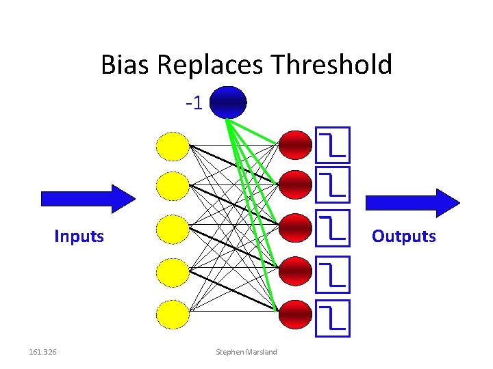
Bias Replaces Threshold -1 Inputs 161. 326 Outputs Stephen Marsland


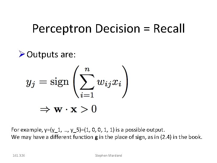
Perceptron Decision = Recall Outputs are: For example, y=(y_1, …, y_5)=(1, 0, 0, 1, 1) is a possible output. We may have a different function g in the place of sign, as in (2. 4) in the book. 161. 326 Stephen Marsland

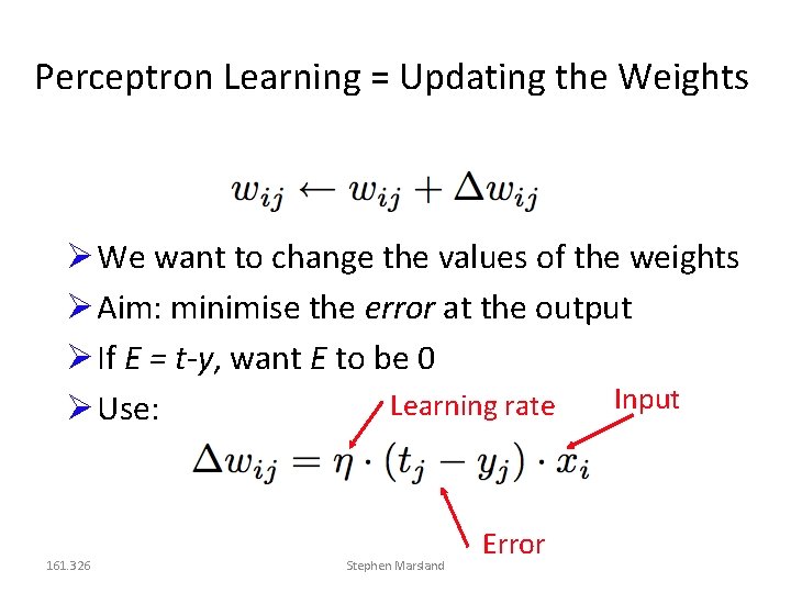
Perceptron Learning = Updating the Weights We want to change the values of the weights Aim: minimise the error at the output If E = t-y, want E to be 0 Input Learning rate Use: 161. 326 Stephen Marsland Error

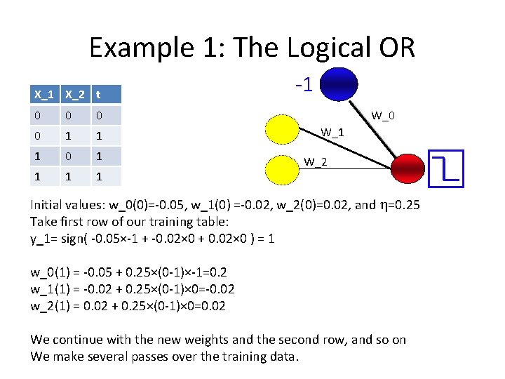
Example 1: The Logical OR X_1 X_2 t 0 0 1 1 1 0 1 1 -1 W_0 W_1 W_2 Initial values: w_0(0)=-0. 05, w_1(0) =-0. 02, w_2(0)=0. 02, and =0. 25 Take first row of our training table: y_1= sign( -0. 05×-1 + -0. 02× 0 + 0. 02× 0 ) = 1 w_0(1) = -0. 05 + 0. 25×(0 -1)×-1=0. 2 w_1(1) = -0. 02 + 0. 25×(0 -1)× 0=-0. 02 w_2(1) = 0. 02 + 0. 25×(0 -1)× 0=0. 02 We continue with the new weights and the second row, and so on We make several passes over the training data.

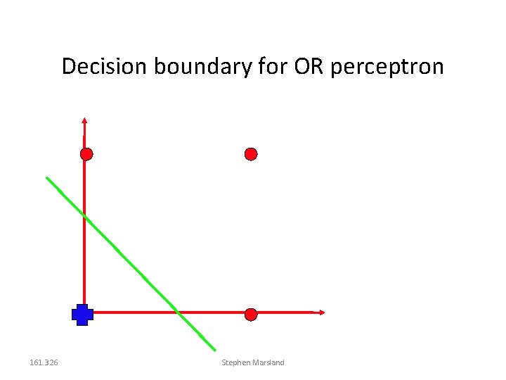
Decision boundary for OR perceptron 161. 326 Stephen Marsland

Perceptron Learning Applet • http: //lcn. epfl. ch/tutorial/english/perceptron/ html/index. html

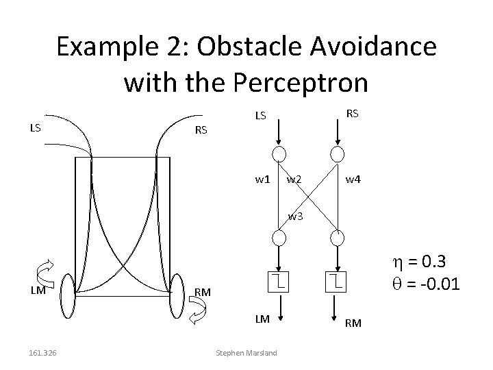
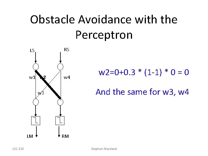
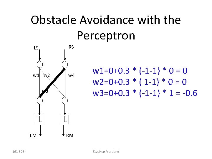
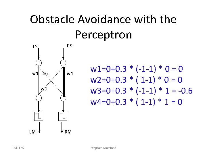
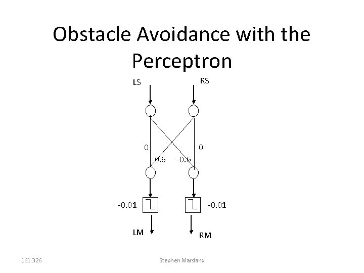
Example 2: Obstacle Avoidance with the Perceptron LS RS RS LS w 1 w 2 w 4 w 3 LM = 0. 3 = -0. 01 RM LM 161. 326 Stephen Marsland RM

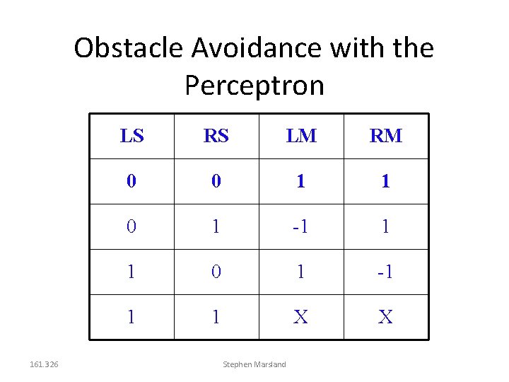
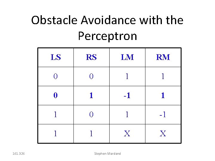
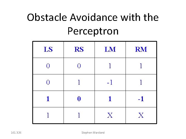
Obstacle Avoidance with the Perceptron 161. 326 LS RS LM RM 0 0 1 1 0 1 -1 1 1 X X Stephen Marsland

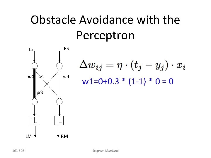
Obstacle Avoidance with the Perceptron LS RS w 1 w 2 w 4 w 1=0+0. 3 * (1 -1) * 0 = 0 w 3 LM 161. 326 RM Stephen Marsland

Obstacle Avoidance with the Perceptron RS LS w 1 w 2 w 4 And the same for w 3, w 4 w 3 LM 161. 326 w 2=0+0. 3 * (1 -1) * 0 = 0 RM Stephen Marsland

Obstacle Avoidance with the Perceptron 161. 326 LS RS LM RM 0 0 1 1 0 1 -1 1 1 X X Stephen Marsland

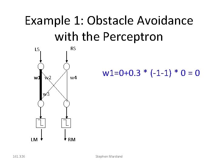
Example 1: Obstacle Avoidance with the Perceptron LS RS w 1 w 2 w 4 w 1=0+0. 3 * (-1 -1) * 0 = 0 w 3 LM 161. 326 RM Stephen Marsland

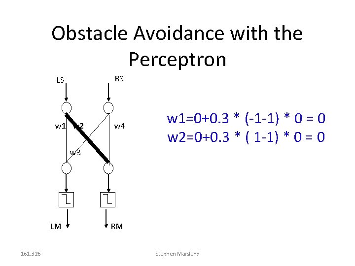
Obstacle Avoidance with the Perceptron LS RS w 1 w 2 w 4 w 1=0+0. 3 * (-1 -1) * 0 = 0 w 2=0+0. 3 * ( 1 -1) * 0 = 0 w 3 LM 161. 326 RM Stephen Marsland

Obstacle Avoidance with the Perceptron LS RS w 1 w 2 w 4 w 3 LM 161. 326 w 1=0+0. 3 * (-1 -1) * 0 = 0 w 2=0+0. 3 * ( 1 -1) * 0 = 0 w 3=0+0. 3 * (-1 -1) * 1 = -0. 6 RM Stephen Marsland

Obstacle Avoidance with the Perceptron LS RS w 1 w 2 w 4 w 3 LM 161. 326 w 1=0+0. 3 * (-1 -1) * 0 = 0 w 2=0+0. 3 * ( 1 -1) * 0 = 0 w 3=0+0. 3 * (-1 -1) * 1 = -0. 6 w 4=0+0. 3 * ( 1 -1) * 1 = 0 RM Stephen Marsland

Obstacle Avoidance with the Perceptron 161. 326 LS RS LM RM 0 0 1 1 0 1 -1 1 1 X X Stephen Marsland

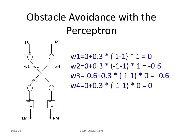
Obstacle Avoidance with the Perceptron RS LS w 1 w 2 w 4 w 3 LM 161. 326 w 1=0+0. 3 * ( 1 -1) * 1 = 0 w 2=0+0. 3 * (-1 -1) * 1 = -0. 6 w 3=-0. 6+0. 3 * ( 1 -1) * 0 = -0. 6 w 4=0+0. 3 * (-1 -1) * 0 = 0 RM Stephen Marsland

Obstacle Avoidance with the Perceptron RS LS 0 0 -0. 6 -0. 01 LM 161. 326 -0. 01 RM Stephen Marsland

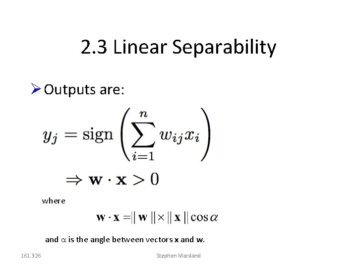
2. 3 Linear Separability Outputs are: where and is the angle between vectors x and w. 161. 326 Stephen Marsland

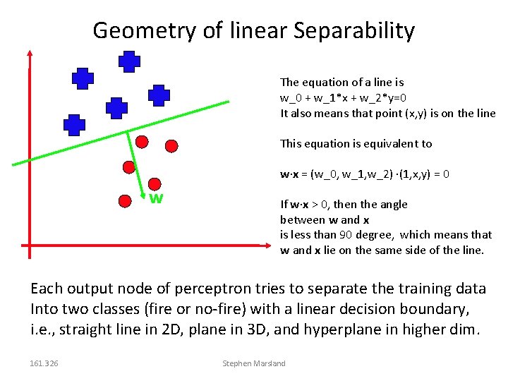
Geometry of linear Separability The equation of a line is w_0 + w_1*x + w_2*y=0 It also means that point (x, y) is on the line This equation is equivalent to w x = (w_0, w_1, w_2) (1, x, y) = 0 w If w x > 0, then the angle between w and x is less than 90 degree, which means that w and x lie on the same side of the line. Each output node of perceptron tries to separate the training data Into two classes (fire or no-fire) with a linear decision boundary, i. e. , straight line in 2 D, plane in 3 D, and hyperplane in higher dim. 161. 326 Stephen Marsland

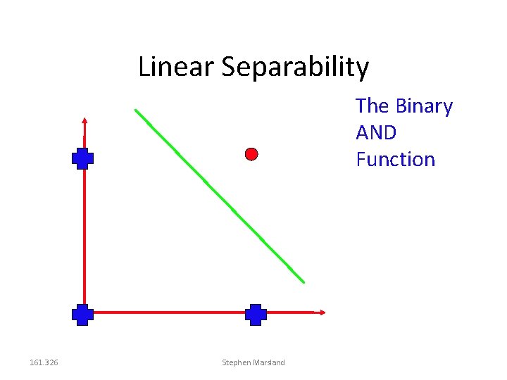
Linear Separability The Binary AND Function 161. 326 Stephen Marsland

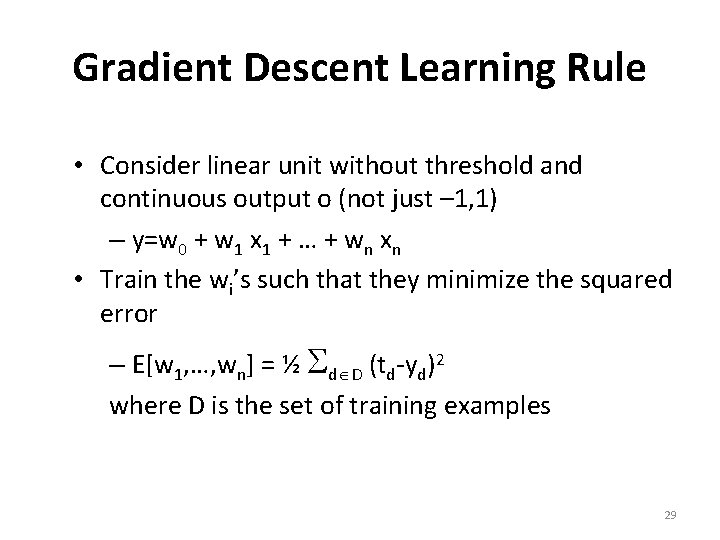
Gradient Descent Learning Rule • Consider linear unit without threshold and continuous output o (not just – 1, 1) – y=w 0 + w 1 x 1 + … + wn xn • Train the wi’s such that they minimize the squared error – E[w 1, …, wn] = ½ d D (td-yd)2 where D is the set of training examples 29

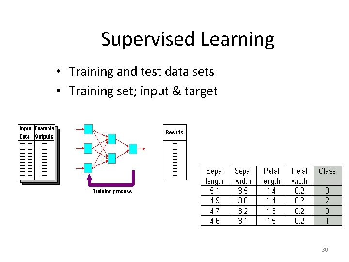
Supervised Learning • Training and test data sets • Training set; input & target 30

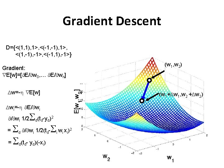
Gradient Descent D={<(1, 1), 1>, <(-1, -1), 1>, <(1, -1), -1>, <(-1, 1), -1>} (w 1, w 2) Gradient: E[w]=[ E/ w 0, … E/ wn] w=- E[w] (w 1+ w 1, w 2 + w 2) wi=- E/ wi (t -y ) = / w 1/2(t - w x ) = (t - y )(-x ) / wi 1/2 d d d i d d d 2 i i i 2 i 31

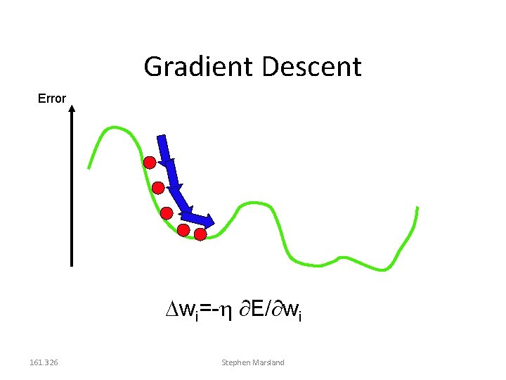
Gradient Descent Error wi=- E/ wi 161. 326 Stephen Marsland
![Incremental Stochastic Gradient Descent Batch mode gradient descent ww EDw over Incremental Stochastic Gradient Descent • Batch mode : gradient descent w=w - ED[w] over](https://slidetodoc.com/presentation_image/4d6ab29cdec775acee6d7b5bb0440b94/image-33.jpg)
Incremental Stochastic Gradient Descent • Batch mode : gradient descent w=w - ED[w] over the entire data D ED[w]=1/2 d(td-yd)2 • Incremental mode: gradient descent w=w - Ed[w] over individual training examples d Ed[w]=1/2 (td-yd)2 Incremental Gradient Descent can approximate Batch Gradient Descent arbitrarily closely if is small enough 33

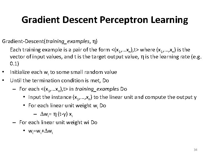
Gradient Descent Perceptron Learning Gradient-Descent(training_examples, ) Each training example is a pair of the form <(x 1, …xn), t> where (x 1, …, xn) is the vector of input values, and t is the target output value, is the learning rate (e. g. 0. 1) • Initialize each wi to some small random value • Until the termination condition is met, Do – For each <(x 1, …xn), t> in training_examples Do • Input the instance (x 1, …, xn) to the linear unit and compute the output y • For each linear unit weight wi Do – wi= (t-y) xi – For each linear unit weight wi Do • wi=wi+ wi 34

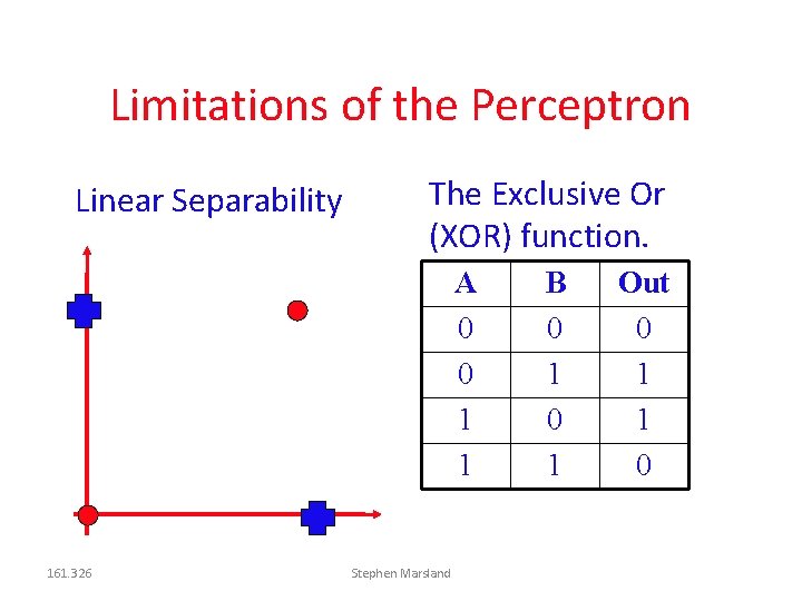
Limitations of the Perceptron Linear Separability The Exclusive Or (XOR) function. A 0 0 1 1 161. 326 Stephen Marsland B 0 1 Out 0 1 1 0

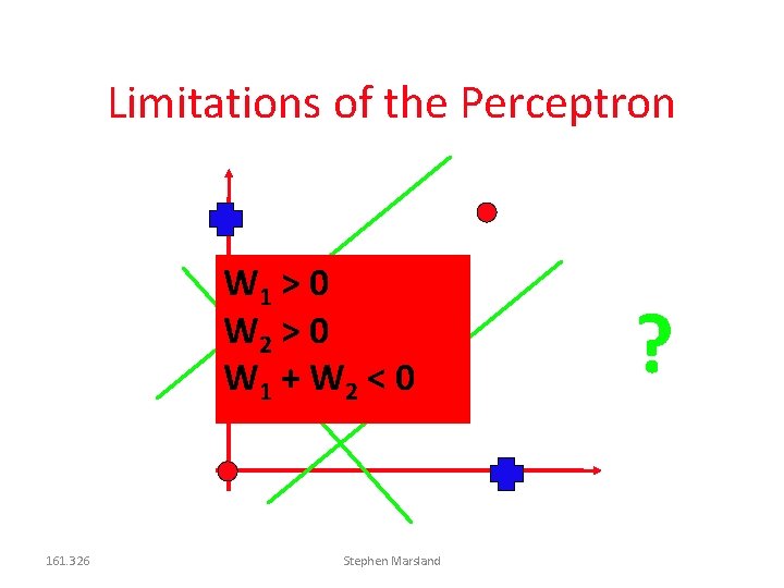
Limitations of the Perceptron W 1 > 0 W 2 > 0 W 1 + W 2 < 0 161. 326 Stephen Marsland ?

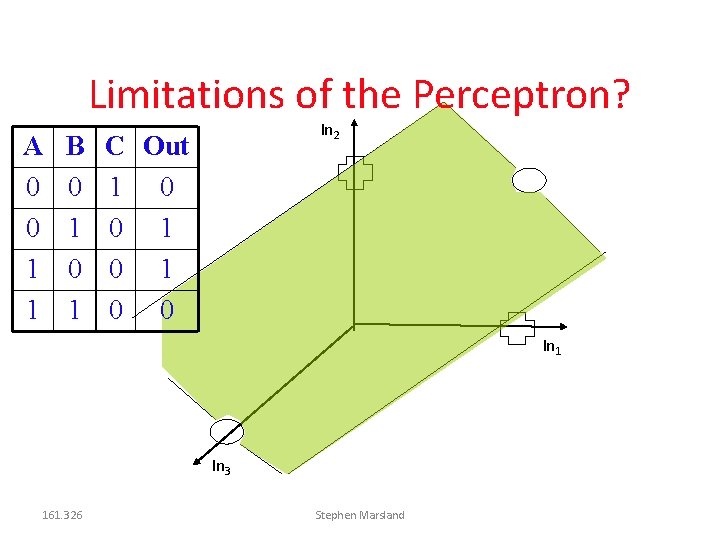
Limitations of the Perceptron? A 0 0 1 1 B 0 1 In 2 C Out 1 0 0 In 1 In 3 161. 326 Stephen Marsland

2. 4 Linear regression Temperature 40 20 26 24 22 20 30 40 20 0 0 20 10 10 20 Given examples Predict 30 given a new point 0 10 0

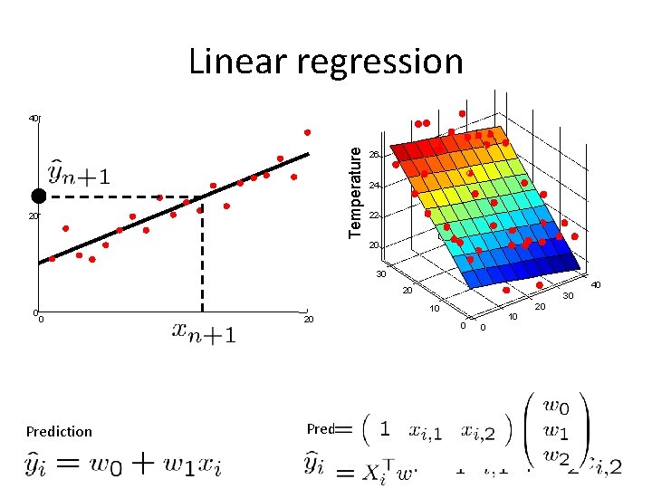
Linear regression Temperature 40 20 26 24 22 20 30 40 20 0 0 Prediction 30 20 10 20 Prediction 0 10 0

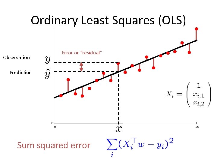
Ordinary Least Squares (OLS) Error or “residual” Observation Prediction 0 0 Sum squared error 20

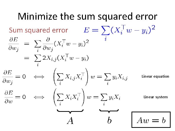
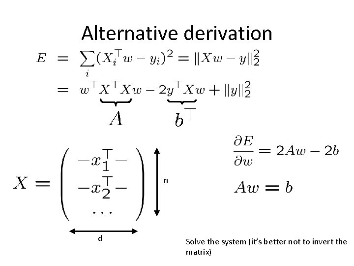
Minimize the sum squared error Sum squared error Linear equation Linear system

Alternative derivation n d Solve the system (it’s better not to invert the matrix)

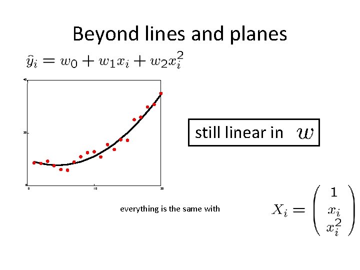
Beyond lines and planes 40 still linear in 20 0 0 10 20 everything is the same with

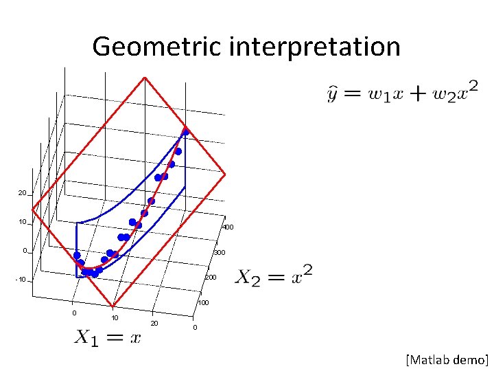
Geometric interpretation 20 10 400 0 300 200 -10 100 0 10 20 0 [Matlab demo]
![Ordinary Least Squares summary Given examples Let For example Let n d Minimize Predict Ordinary Least Squares [summary] Given examples Let For example Let n d Minimize Predict](https://slidetodoc.com/presentation_image/4d6ab29cdec775acee6d7b5bb0440b94/image-45.jpg)
Ordinary Least Squares [summary] Given examples Let For example Let n d Minimize Predict by solving

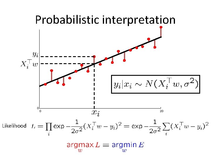
Probabilistic interpretation 0 Likelihood 0 20

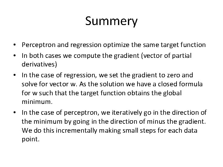
Summery • Perceptron and regression optimize the same target function • In both cases we compute the gradient (vector of partial derivatives) • In the case of regression, we set the gradient to zero and solve for vector w. As the solution we have a closed formula for w such that the target function obtains the global minimum. • In the case of perceptron, we iteratively go in the direction of the minimum by going in the direction of minus the gradient. We do this incrementally making small steps for each data point.

Homework 1 • (Ch. 2. 3. 3) Implement perceptron in Matlab and test it on the Pmia Indian Dataset from UCI Machine Learning Repository: http: //archive. ics. uci. edu/ml/ • (Ch. 2. 4. 1) Implementing linear regression in Matlab and apply it to auto-mpg dataset.

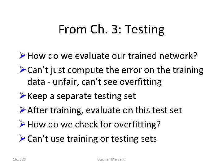
From Ch. 3: Testing How do we evaluate our trained network? Can’t just compute the error on the training data - unfair, can’t see overfitting Keep a separate testing set After training, evaluate on this test set How do we check for overfitting? Can’t use training or testing sets 161. 326 Stephen Marsland

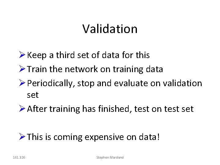
Validation Keep a third set of data for this Train the network on training data Periodically, stop and evaluate on validation set After training has finished, test on test set This is coming expensive on data! 161. 326 Stephen Marsland

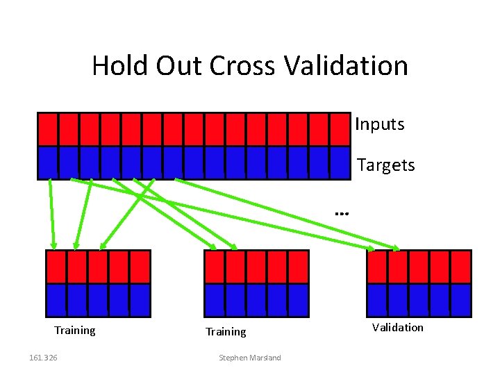
Hold Out Cross Validation Inputs Targets … Training 161. 326 Training Stephen Marsland Validation

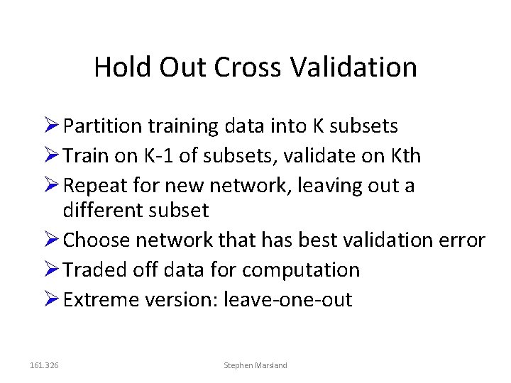
Hold Out Cross Validation Partition training data into K subsets Train on K-1 of subsets, validate on Kth Repeat for new network, leaving out a different subset Choose network that has best validation error Traded off data for computation Extreme version: leave-one-out 161. 326 Stephen Marsland

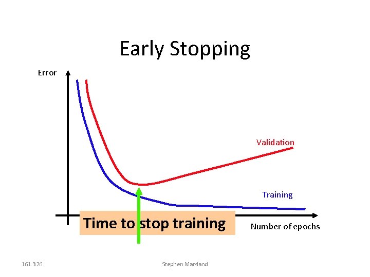
Early Stopping When should we stop training? Could set a minimum training error Danger of overfitting Could set a number of epochs Danger of underfitting or overfitting Can use the validation set Measure the error on the validation set during training 161. 326 Stephen Marsland

Early Stopping Error Validation Training Time to stop training 161. 326 Stephen Marsland Number of epochs