Ch 2 4 Differences Between Linear and Nonlinear
Ch 2. 4: Differences Between Linear and Nonlinear Equations Recall that a first order ODE has the form y' = f (t, y), and is linear if f is linear in y, and nonlinear if f is nonlinear in y. Examples: y' = t y - e t, y' = t y 2. In this section, we will see that first order linear and nonlinear equations differ in a number of ways, including: The theory describing existence and uniqueness of solutions, and corresponding domains, are different. Solutions to linear equations can be expressed in terms of a general solution, which is not usually the case for nonlinear equations. Linear equations have explicitly defined solutions while nonlinear equations typically do not, and nonlinear equations may or may not have implicitly defined solutions.
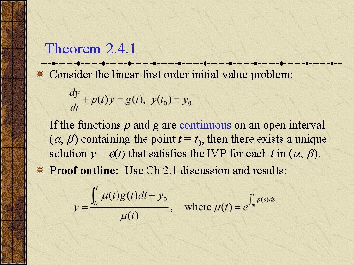
Theorem 2. 4. 1 Consider the linear first order initial value problem: If the functions p and g are continuous on an open interval ( , ) containing the point t = t 0, then there exists a unique solution y = (t) that satisfies the IVP for each t in ( , ). Proof outline: Use Ch 2. 1 discussion and results:
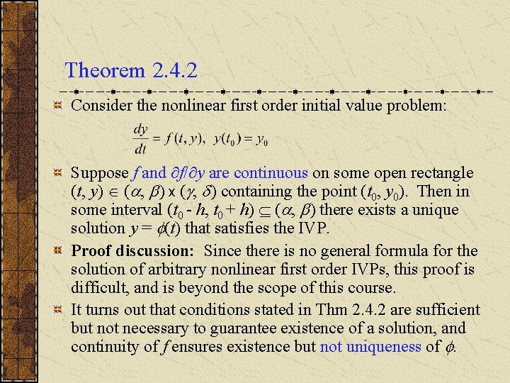
Theorem 2. 4. 2 Consider the nonlinear first order initial value problem: Suppose f and f/ y are continuous on some open rectangle (t, y) ( , ) x ( , ) containing the point (t 0, y 0). Then in some interval (t 0 - h, t 0 + h) ( , ) there exists a unique solution y = (t) that satisfies the IVP. Proof discussion: Since there is no general formula for the solution of arbitrary nonlinear first order IVPs, this proof is difficult, and is beyond the scope of this course. It turns out that conditions stated in Thm 2. 4. 2 are sufficient but not necessary to guarantee existence of a solution, and continuity of f ensures existence but not uniqueness of .
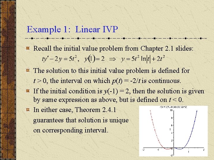
Example 1: Linear IVP Recall the initial value problem from Chapter 2. 1 slides: The solution to this initial value problem is defined for t > 0, the interval on which p(t) = -2/t is continuous. If the initial condition is y(-1) = 2, then the solution is given by same expression as above, but is defined on t < 0. In either case, Theorem 2. 4. 1 guarantees that solution is unique on corresponding interval.
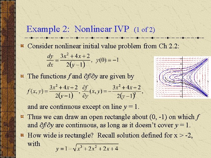
Example 2: Nonlinear IVP (1 of 2) Consider nonlinear initial value problem from Ch 2. 2: The functions f and f/ y are given by and are continuous except on line y = 1. Thus we can draw an open rectangle about (0, -1) on which f and f/ y are continuous, as long as it doesn’t cover y = 1. How wide is rectangle? Recall solution defined for x > -2, with
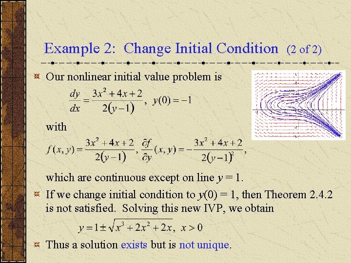
Example 2: Change Initial Condition (2 of 2) Our nonlinear initial value problem is with which are continuous except on line y = 1. If we change initial condition to y(0) = 1, then Theorem 2. 4. 2 is not satisfied. Solving this new IVP, we obtain Thus a solution exists but is not unique.
- Slides: 6