CH 12 Cost of Capital and Valuation Basics

Topics • Present Value Review • Cost of Capital • Dividend Discount Model

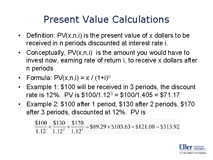
Present Value Calculations • Definition: PV(x, n, i) is the present value of x dollars to be received in n periods discounted at interest rate i. • Conceptually, PV(x, n, i) is the amount you would have to invest now, earning rate of return i, to receive x dollars after n periods • Formula: PV(x, n, i) = x / (1+i)n • Example 1: $100 will be received in 3 periods, the discount rate is 12%. PV is $100/1. 123 = $100/1. 405 = $71. 17 • Example 2: $100 after 1 period, $130 after 2 periods, $170 after 3 periods, discounted at 12%. PV is

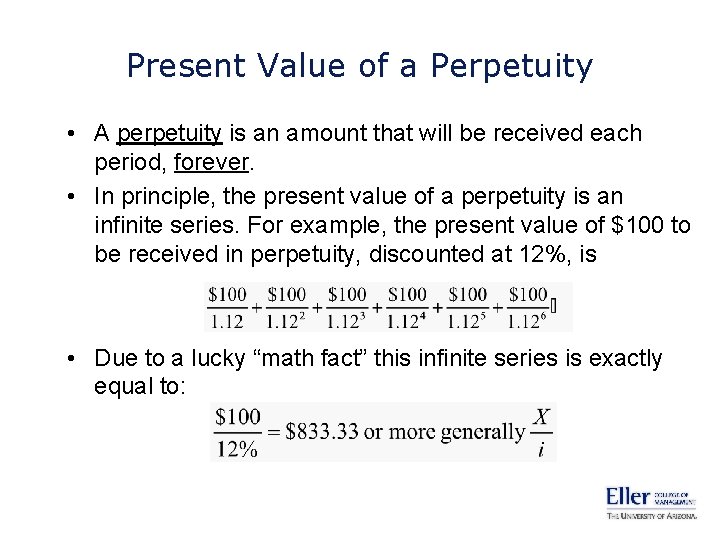
Present Value of a Perpetuity • A perpetuity is an amount that will be received each period, forever. • In principle, the present value of a perpetuity is an infinite series. For example, the present value of $100 to be received in perpetuity, discounted at 12%, is • Due to a lucky “math fact” this infinite series is exactly equal to:

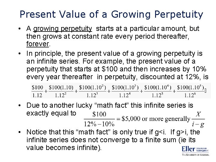
Present Value of a Growing Perpetuity • A growing perpetuity starts at a particular amount, but then grows at constant rate every period thereafter, forever. • In principle, the present value of a growing perpetuity is an infinite series. For example, the present value of a perpetuity that starts at $100 and then increases by 10% every year thereafter in perpetuity, discounted at 12%, is • Due to another lucky “math fact” this infinite series is exactly equal to • Notice that this “math fact” is only true if g<i. If g>i, the infinite series does not converge to a finite sum (ie its value becomes infinite).

Cost of Capital • The term “cost of capital” refers to the rate of return capital providers demand in order to provide money to the firm. • For debt: effective interest rate. • Preferred stock: dividend yield. • Equity: Use expected rate of return according to Capital Asset Pricing Model (CAPM)

Beta and the Cost of Equity Capital • The central theory in the field of finance is the “Capital Asset Pricing Model” or “CAPM. ” • CAPM says the return you should expect to earn on a stock depends on its Beta: E(Ri) = Rf + β[E(Rm)-Rf] where Rf is the risk-free interest rate, and [E(Rm)-Rf] is called the “market risk premium. ” • If the market risk premium is around 6%, the firm has β=1. 5 and Rf=3%, then E(Ri) =3%+1. 5*6%=12%. • Data Needed: Beta, Risk-Free Rate, Market Risk Premium

Beta • Beta is a statistic that measures how the firm’s stock price moves with the market. • If the market index changes by 1%, does the firm’s stock price change (on average) by ½%? by 1%? by 2%? Beta in these three cases is 0. 5, 1. 0 and 2. 0 • The higher Beta is, the higher the firm’s systematic risk is. • The firm’s stock price can also change for reasons unrelated to changes in the market. This kind of risk is called “nonsystematic” or “idiosyncratic” or “unique” or “diversifiable” • Beta is usually estimated empirically using regression analysis.

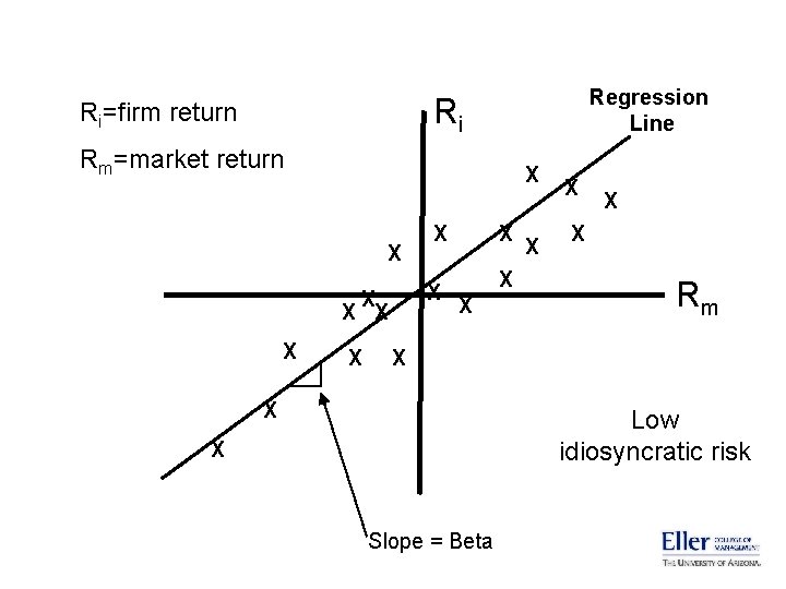
Regression Line Ri Ri=firm return Rm=market return X X X X Rm X X Low idiosyncratic risk X Slope = Beta

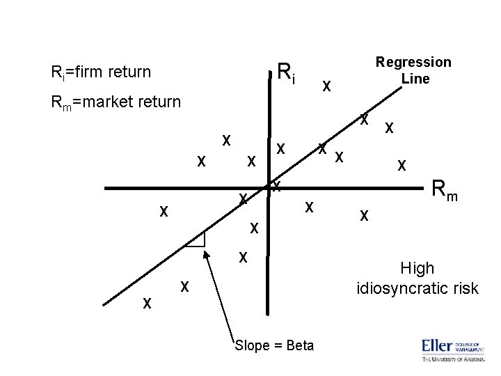
Ri Ri=firm return X Rm=market return X X X Slope = Beta X X Rm X X X Regression Line X High idiosyncratic risk

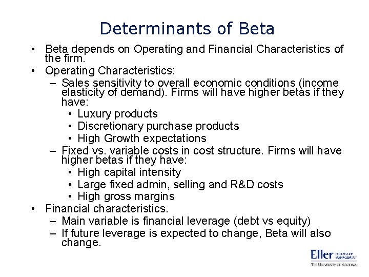
Determinants of Beta • Beta depends on Operating and Financial Characteristics of the firm. • Operating Characteristics: – Sales sensitivity to overall economic conditions (income elasticity of demand). Firms will have higher betas if they have: • Luxury products • Discretionary purchase products • High Growth expectations – Fixed vs. variable costs in cost structure. Firms will have higher betas if they have: • High capital intensity • Large fixed admin, selling and R&D costs • High gross margins • Financial characteristics. – Main variable is financial leverage (debt vs equity) – If future leverage is expected to change, Beta will also change.

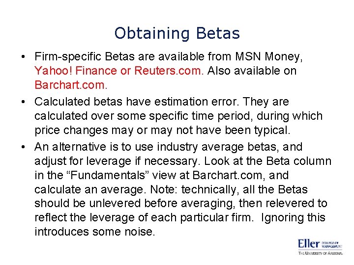
Obtaining Betas • Firm-specific Betas are available from MSN Money, Yahoo! Finance or Reuters. com. Also available on Barchart. com. • Calculated betas have estimation error. They are calculated over some specific time period, during which price changes may or may not have been typical. • An alternative is to use industry average betas, and adjust for leverage if necessary. Look at the Beta column in the “Fundamentals” view at Barchart. com, and calculate an average. Note: technically, all the Betas should be unlevered before averaging, then relevered to reflect the leverage of each particular firm. Ignoring this introduces some noise.

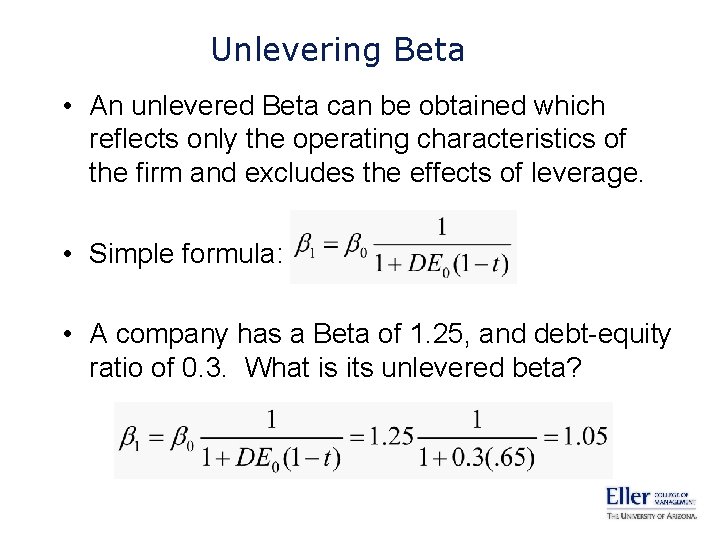
Unlevering Beta • An unlevered Beta can be obtained which reflects only the operating characteristics of the firm and excludes the effects of leverage. • Simple formula: • A company has a Beta of 1. 25, and debt-equity ratio of 0. 3. What is its unlevered beta?

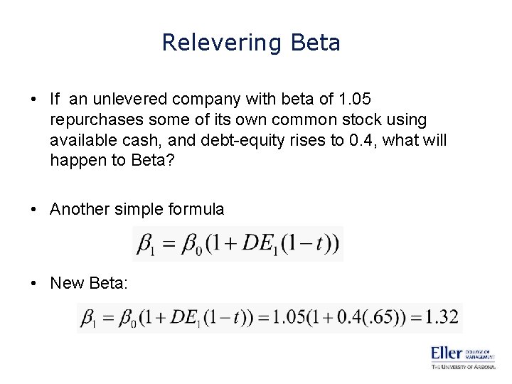
Relevering Beta • If an unlevered company with beta of 1. 05 repurchases some of its own common stock using available cash, and debt-equity rises to 0. 4, what will happen to Beta? • Another simple formula • New Beta:

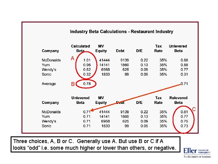
A B C Three choices, A, B or C. Generally use A. But use B or C if A looks “odd” i. e. some much higher or lower than others, or negative.

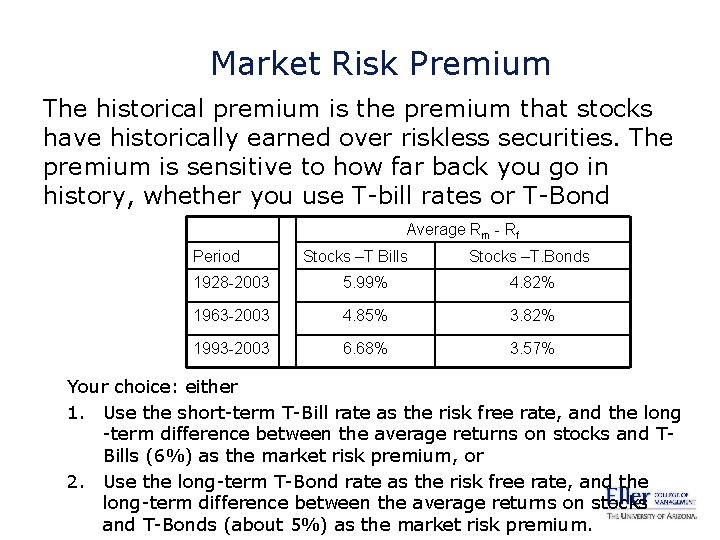
Market Risk Premium The historical premium is the premium that stocks have historically earned over riskless securities. The premium is sensitive to how far back you go in history, whether you use T-bill rates or T-Bond Average Rm - Rf Period Stocks –T Bills Stocks –T. Bonds 1928 -2003 5. 99% 4. 82% 1963 -2003 4. 85% 3. 82% 1993 -2003 6. 68% 3. 57% Your choice: either 1. Use the short-term T-Bill rate as the risk free rate, and the long -term difference between the average returns on stocks and TBills (6%) as the market risk premium, or 2. Use the long-term T-Bond rate as the risk free rate, and the long-term difference between the average returns on stocks and T-Bonds (about 5%) as the market risk premium.

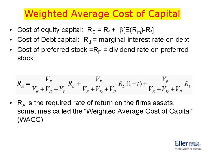
Weighted Average Cost of Capital • Cost of equity capital: RE = Rf + [E(Rm)-Rf] • Cost of Debt capital: Rd = marginal interest rate on debt • Cost of preferred stock =RP = dividend rate on preferred stock. • RA is the required rate of return on the firms assets, sometimes called the “Weighted Average Cost of Capital” (WACC)

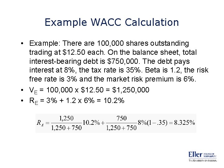
Example WACC Calculation • Example: There are 100, 000 shares outstanding trading at $12. 50 each. On the balance sheet, total interest-bearing debt is $750, 000. The debt pays interest at 8%, the tax rate is 35%. Beta is 1. 2, the risk free rate is 3% and the market risk premium is 6%. • VE = 100, 000 x $12. 50 = $1, 250, 000 • RE = 3% + 1. 2 x 6% = 10. 2%

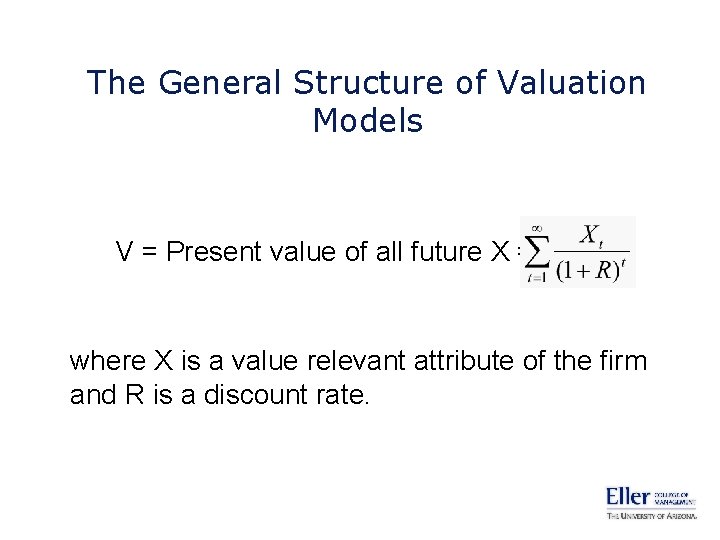
The General Structure of Valuation Models V = Present value of all future X = where X is a value relevant attribute of the firm and R is a discount rate.

Requirements for practical application of valuation models • We need to decide what X is. • We can’t forecast to infinity, so we have to find a way of adapting the formula to a finite period. (This is referred to as a “terminal value assumption”) • We need to know what discount rate is appropriate: – Cost of equity capital if X is claimed entirely by equity holders. – WACC if X is claimed by equity, debt and preferred holders

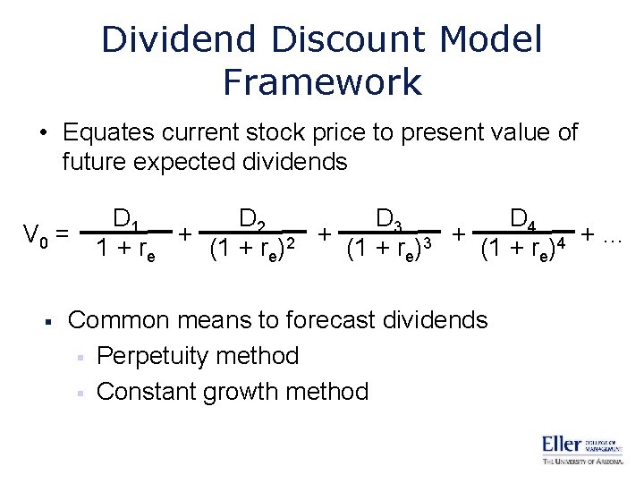
Dividend Discount Model Framework • Equates current stock price to present value of future expected dividends V 0 = § D 1 D 2 D 3 D 4 + +… 2 3 4 1 + re (1 + re) Common means to forecast dividends § Perpetuity method § Constant growth method

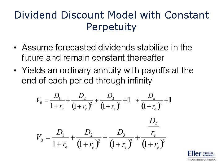
Dividend Discount Model with Constant Perpetuity • Assume forecasted dividends stabilize in the future and remain constant thereafter • Yields an ordinary annuity with payoffs at the end of each period through infinity

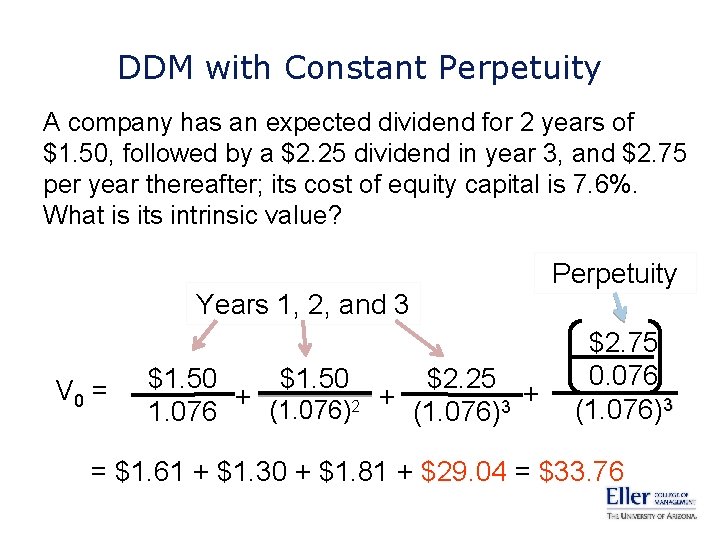
DDM with Constant Perpetuity A company has an expected dividend for 2 years of $1. 50, followed by a $2. 25 dividend in year 3, and $2. 75 per year thereafter; its cost of equity capital is 7. 6%. What is its intrinsic value? Years 1, 2, and 3 V 0 = $1. 50 $2. 25 + + (1. 076)2 + 3 1. 076 (1. 076) Perpetuity $2. 75 0. 076 (1. 076)3 = $1. 61 + $1. 30 + $1. 81 + $29. 04 = $33. 76

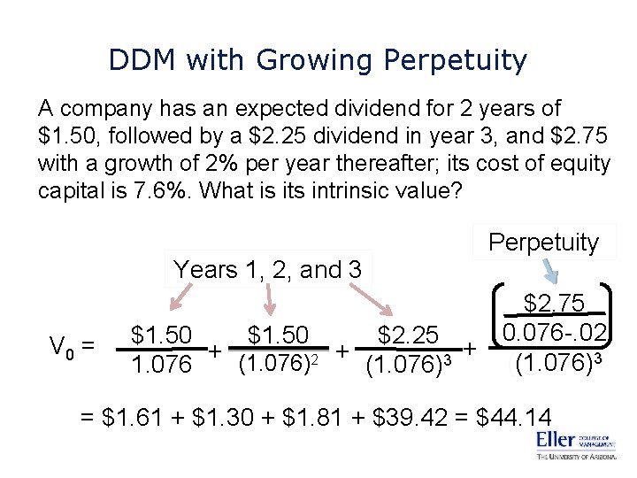
DDM with Growing Perpetuity A company has an expected dividend for 2 years of $1. 50, followed by a $2. 25 dividend in year 3, and $2. 75 with a growth of 2% per year thereafter; its cost of equity capital is 7. 6%. What is its intrinsic value? Years 1, 2, and 3 V 0 = $1. 50 $2. 25 + + (1. 076)2 + 3 1. 076 (1. 076) Perpetuity $2. 75 0. 076 -. 02 ((1. 076)3 = $1. 61 + $1. 30 + $1. 81 + $39. 42 = $44. 14

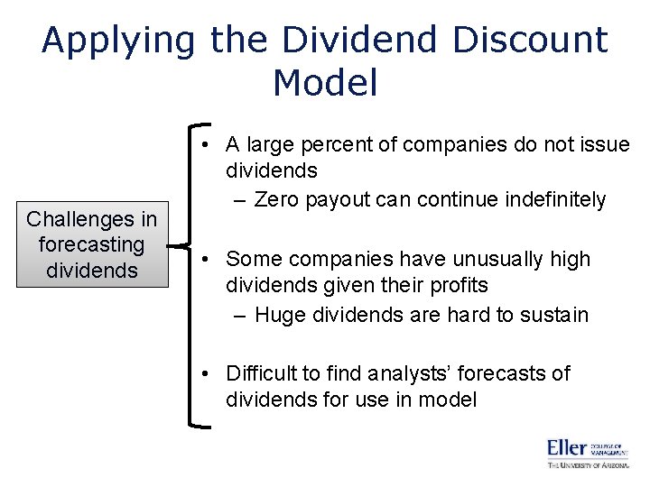
Applying the Dividend Discount Model Challenges in forecasting dividends • A large percent of companies do not issue dividends – Zero payout can continue indefinitely • Some companies have unusually high dividends given their profits – Huge dividends are hard to sustain • Difficult to find analysts’ forecasts of dividends for use in model