Centralized Query Optimization Group 2 03 Pruthvi Pulluru

Centralized Query Optimization Group 2 #03 Pruthvi Pulluru #19 Sarath Dammu #15 Raja Shekar Reddy Pandiri #11 Naga Krishna Ganta #14 Neelima Devi Arigala Instructor: Morris Liaw

CONTENTS • DYNAMIC QUERY OPTIMIZATION • ALGORITHM FOR DYNAMIC-QOA • STATIC QUERY OPTIMIZATION • ALGORITHM FOR STATIC-QOA • HYBRID QUERY OPTIMIZATION

Example 8. 4. To illustrate the detachment technique, we apply it to the following query: “Names of employees working on the CAD/CAM project” This query can be expressed in SQL by the following query q 1: SELECT EMP. ENAME FROM EMP, ASG, PROJ WHERE EMP. ENO=ASG. ENO AND ASG. PNO=PROJ. PNO AND PNAME="CAD/CAM" After detachment of the selections, query q 1 is replaced by q 11 followed by q 0, where JVAR is an intermediate relation.

q 11: SELECT PROJ. PNO INTO JVAR FROM PROJ WHERE PNAME="CAD/CAM" q 0: SELECT EMP. ENAME FROM EMP, ASG, JVAR WHERE EMP. ENO=ASG. ENO AND ASG. PNO=JVAR. PNO The successive detachments of q 0 may generate q 12: SELECT ASG. ENO INTO GVAR FROM ASG, JVAR WHERE ASG. PNO=JVAR. PNO q 13: SELECT EMP. ENAME FROM EMP, GVAR WHERE EMP. ENO=GVAR. ENO

• QUERY Q 11 IS MONO RELATION AND CAN BE EXECUTED. HOWEVER, Q 12 AND Q 13 ARE NOT MONO RELATION AND CANNOT BE REDUCED BY DETACHMENT. • MULTI RELATION QUERIES, WHICH CANNOT BE FURTHER DETACHED (E. G. , Q 12 AND Q 13), ARE IRREDUCIBLE. • A QUERY IS IRREDUCIBLE IF AND ONLY IF ITS QUERY GRAPH IS A CHAIN WITH TWO NODES OR A CYCLE WITH K NODES WHERE K > 2. IRREDUCIBLE QUERIES ARE CONVERTED INTO MONO RELATION QUERIES BY TUPLE SUBSTITUTION.

Multi relation queries, which cannot be further detached (e. g. , q 12 and q 13), are irreducible. A query is irreducible if and only if its query graph is a chain with two nodes or a cycle with k nodes where k > 2. Irreducible queries are converted into Mono relation queries by tuple substitution. Given an n-relation query q, the tuples of one relation are substituted by their values, thereby producing a set of (n-1)relation queries. Tuple substitution proceeds as follows. First, one relation in q is chosen for tuple substitution. Let R 1 be that relation. Then for each tuple t 1 i in R 1, the attributes referred to by in q are replaced by their actual values in t 1 i, thereby generating a query q 0 with n-1 relations.

Therefore, the total number of queries q 0 produced by tuple substitution is card(R 1). Tuple substitution can be summarized as follows: q(R 1; R 2; : : : ; Rn) is replaced by fq 0(t 1 i; R 2; R 3; : : : ; Rn); t 1 i 2 R 1 g For each tuple thus obtained, the subquery is recursively processed by substitution if it is not yet irreducible.

Example 8. 5. Let us consider the query q 13: SELECT EMP. ENAME FROM EMP, GVAR WHERE EMP. ENO=GVAR. ENO The relation GVAR is over a single attribute (ENO). Assume that it contains only two tuples: h. E 1 i and h. E 2 i. The substitution of GVAR generates two one-relation subqueries: q 131: SELECT EMP. ENAME FROM EMP WHERE EMP. ENO="E 1" q 132: SELECT EMP. ENAME FROM EMP WHERE EMP. ENO="E 2" These queries may then be executed.

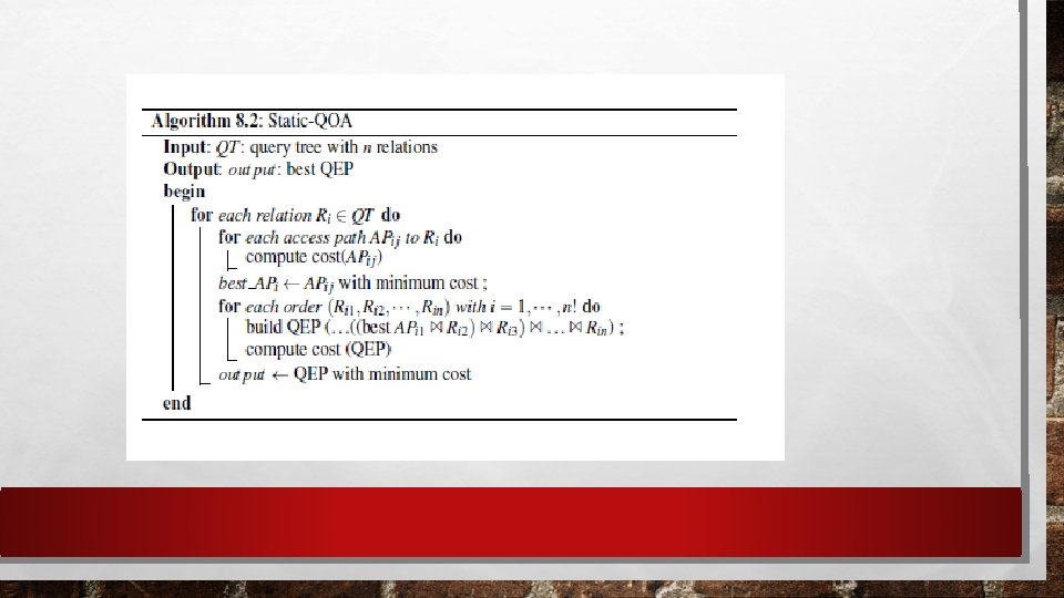
8. 2. 2 Static Query Optimization With static query optimization, there is a clear separation between the generation of the QEP at compile-time and its execution by the DBMS execution engine. Thus, an accurate cost model is key to predict the costs of candidate QEPs. The most popular static query optimization algorithm is that of System R also one of the first relational DBMS. In this section, we present this algorithm based on the description by Selinger et al. [1979].

Most commercial relational DBMSs have implemented variants of this algorithm due to its efficiency and compatibility with query compilation. The input to the optimizer is a relational algebra tree resulting from the decomposition of an SQL query. The output is a QEP that implements the “optimal” relational algebra tree. The optimizer assigns a cost (in terms of time) to every candidate tree and retains the one with the smallest cost.

The candidate trees are obtained by a permutation of the join orders of the n relations of the query using the commutativity and associativity rules. To limit the overhead of optimization, the number of alternative trees is reduced using dynamic programming. The set of alternative strategies is constructed dynamically so that, when two joins are equivalent by commutativity, only the cheapest one is kept. Furthermore, the strategies that include Cartesian products are eliminated whenever possible.

The cost of a candidate strategy is a weighted combination of I/O and CPU costs. The estimation of such costs (at compile time) is based on a cost model that provides a cost formula for each low-level operation (e. g. , select using a Btree index with a range predicate). For most operations (except exact match select), these cost formulas are based on the cardinalities of the operands. The cardinality information for the relations stored in the database is found in the database statistics.

The optimization algorithm consists of two major steps. First, the best access method to each individual relation based on a select predicate is predicted (this is the one with the least cost). Second, for each relation R, the best join ordering is estimated, where R is first accessed using its best single-relation access method. The cheapest ordering becomes the basis for the best execution plan. For the join of two relations, the relation whose tuples are read first is called the external, while the other, whose tuples are found according to the values obtained from the external relation, is called the internal relation. An important decision with either join method is to determine the cheapest access path to the internal relation.

EMP: sequential scan (because there is no selection on EMP) ASG: sequential scan (because there is no selection on ASG) PROJ: index on PNAME (because there is a selection on PROJ based on PNAME)

The dynamic construction of the tree of alternative strategies is illustrated in Figure 8. 9. Note that the maximum number of join orders is 3!; dynamic search considers fewer alternatives, as depicted in Figure 8. 9. The operations marked “pruned” are dynamically eliminated. The first level of the tree indicates the best single-relation access method. The second level indicates, for each of these, the best join method with any other relation. Strategies (EMP * PROJ) and (PROJ * EMP) are pruned because they are Cartesian products that can be avoided (by other strategies).

Select PROJ using index on PNAME Then join with ASG using index on PNO Then join with EMP using index on ENO

Hybrid Query Optimization Dynamic and static query optimimization both have advantages and drawbacks. Dynamic query optimization mixes optimization and execution and thus can make accurate optimization choices at run-time. However, query optimization is repeated for each execution of the query. Therefore, this approach is best for ad-hoc queries. Static query optimization, done at compilation time, amortizes the cost of optimization over multiple query executions.

The accuracy of the cost model is thus critical to predict the costs of candidate QEPs. This approach is best for queries embedded in stored procedures, and has been adopted by all commercial DBMSs. However, even with a sophisticated cost model, there is an important problem that prevents accurate cost estimation and comparison of QEPs at compiletime. The problem is that the actual bindings of parameter values in embedded queries is not known until run-time.

• HYBRID QUERY OPTIMIZATION ATTEMPTS TO PROVIDE THE ADVANTAGES OF STATIC QUERY OPTIMIZATION WHILE AVOIDING THE ISSUES GENERATED BY INACCURATE ESTIMATES. • • THE APPROACHIS BASICALLY STATIC, BUT FURTHER OPTIMIZATION DECISIONS MAY TAKE PLACE AT RUN TIME. THIS APPROACH WAS PIONNERED IN SYSTEM R BY ADDING A CONDITIONAL RUNTIME RE OPTIMIZATION PHASE FOR EXECUTION PLANS STATICALLY OPTIMIZED. • A MORE GENERAL SOLUTION IS TO PRODUCE DYNAMIC QEPS WHICH INCLUDE CAREFULLY SELECTED OPTIMIZATION DECISIONS TO BE MADE AT RUNTIME USING “CHOOSE-PLAN” OPERATORS.