Centrality revisited Degree Centrality how well connected direct

Centrality revisited

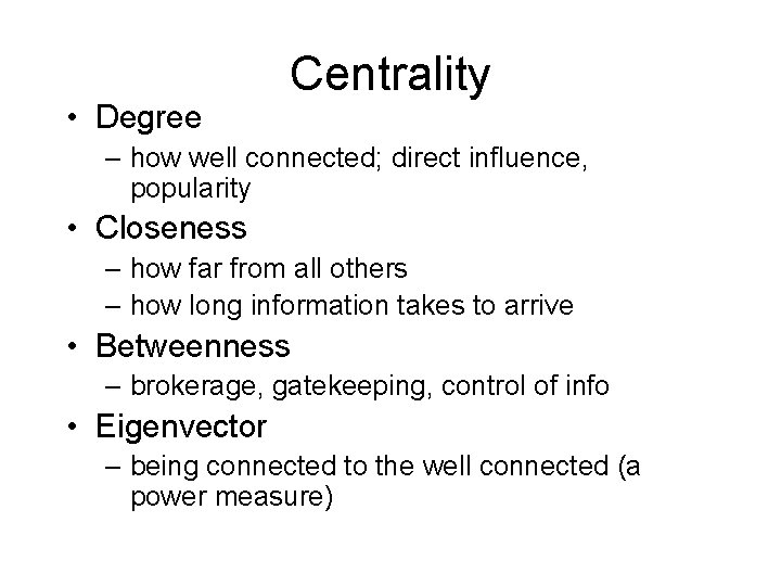
• Degree Centrality – how well connected; direct influence, popularity • Closeness – how far from all others – how long information takes to arrive • Betweenness – brokerage, gatekeeping, control of info • Eigenvector – being connected to the well connected (a power measure)

Data Issues • • Directed data Valued data Disconnected data Negative ties

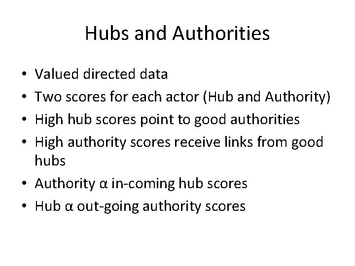
Hubs and Authorities Valued directed data Two scores for each actor (Hub and Authority) High hub scores point to good authorities High authority scores receive links from good hubs • Authority α in-coming hub scores • Hub α out-going authority scores • •

Hubs and Authorities • Generalization of eigenvector centrality • Actually the scores are singular vectors • In UCINET normalized so the sum of squares is one • First major use in page ranking for the www

Krackhardt Advice Data • • • High tech company Who do you go to for advice High hubs know who to go to High authority scores are who you ask A kind of consensus model

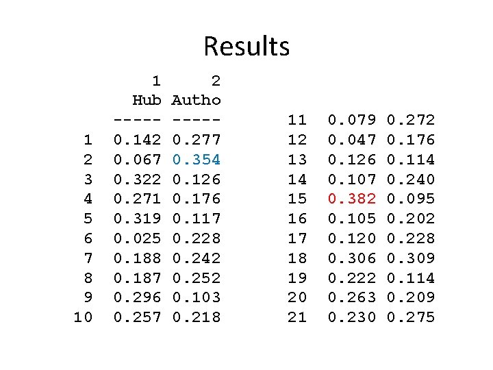
Results 1 2 3 4 5 6 7 8 9 10 1 Hub ----0. 142 0. 067 0. 322 0. 271 0. 319 0. 025 0. 188 0. 187 0. 296 0. 257 2 Autho ----0. 277 0. 354 0. 126 0. 176 0. 117 0. 228 0. 242 0. 252 0. 103 0. 218 11 12 13 14 15 16 17 18 19 20 21 0. 079 0. 047 0. 126 0. 107 0. 382 0. 105 0. 120 0. 306 0. 222 0. 263 0. 230 0. 272 0. 176 0. 114 0. 240 0. 095 0. 202 0. 228 0. 309 0. 114 0. 209 0. 275

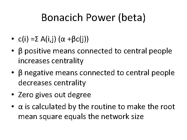
Bonacich Power (beta) • c(i) =Σ A(i, j) (α +βc(j)) • β positive means connected to central people increases centrality • β negative means connected to central people decreases centrality • Zero gives out degree • α is calculated by the routine to make the root mean square equals the network size

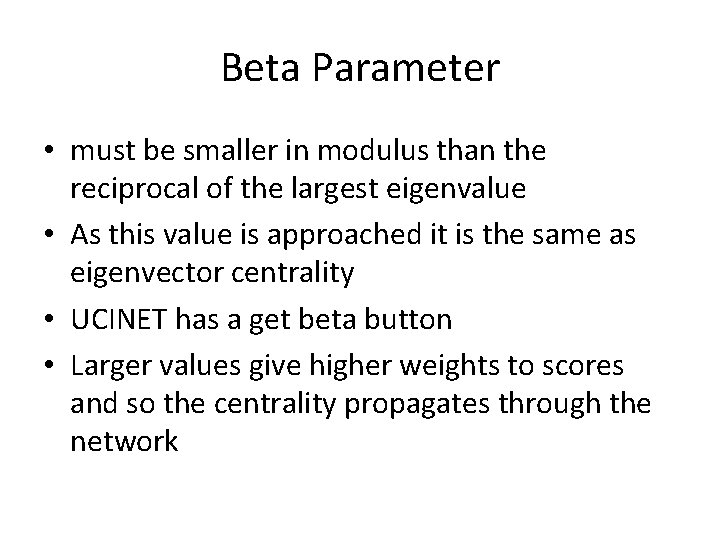
Beta Parameter • must be smaller in modulus than the reciprocal of the largest eigenvalue • As this value is approached it is the same as eigenvector centrality • UCINET has a get beta button • Larger values give higher weights to scores and so the centrality propagates through the network

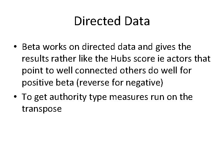
Directed Data • Beta works on directed data and gives the results rather like the Hubs score ie actors that point to well connected others do well for positive beta (reverse for negative) • To get authority type measures run on the transpose

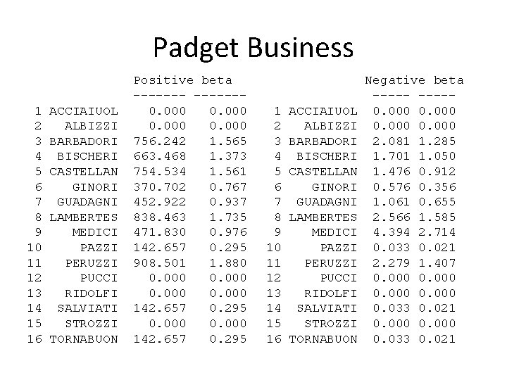
Padget Business 1 2 3 4 5 6 7 8 9 10 11 12 13 14 15 16 ACCIAIUOL ALBIZZI BARBADORI BISCHERI CASTELLAN GINORI GUADAGNI LAMBERTES MEDICI PAZZI PERUZZI PUCCI RIDOLFI SALVIATI STROZZI TORNABUON Positive beta -------0. 000 756. 242 1. 565 663. 468 1. 373 754. 534 1. 561 370. 702 0. 767 452. 922 0. 937 838. 463 1. 735 471. 830 0. 976 142. 657 0. 295 908. 501 1. 880 0. 000 142. 657 0. 295 0. 000 142. 657 0. 295 1 2 3 4 5 6 7 8 9 10 11 12 13 14 15 16 ACCIAIUOL ALBIZZI BARBADORI BISCHERI CASTELLAN GINORI GUADAGNI LAMBERTES MEDICI PAZZI PERUZZI PUCCI RIDOLFI SALVIATI STROZZI TORNABUON Negative beta -----0. 000 2. 081 1. 285 1. 701 1. 050 1. 476 0. 912 0. 576 0. 356 1. 061 0. 655 2. 566 1. 585 4. 394 2. 714 0. 033 0. 021 2. 279 1. 407 0. 000 0. 033 0. 021

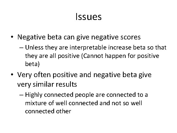
Issues • Negative beta can give negative scores – Unless they are interpretable increase beta so that they are all positive (Cannot happen for positive beta) • Very often positive and negative beta give very similar results – Highly connected people are connected to a mixture of well connected and not so well connected other

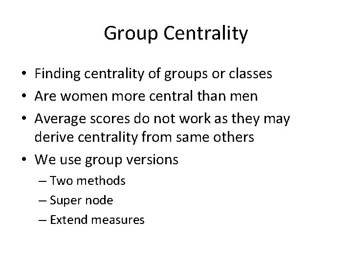
Group Centrality • Finding centrality of groups or classes • Are women more central than men • Average scores do not work as they may derive centrality from same others • We use group versions – Two methods – Super node – Extend measures

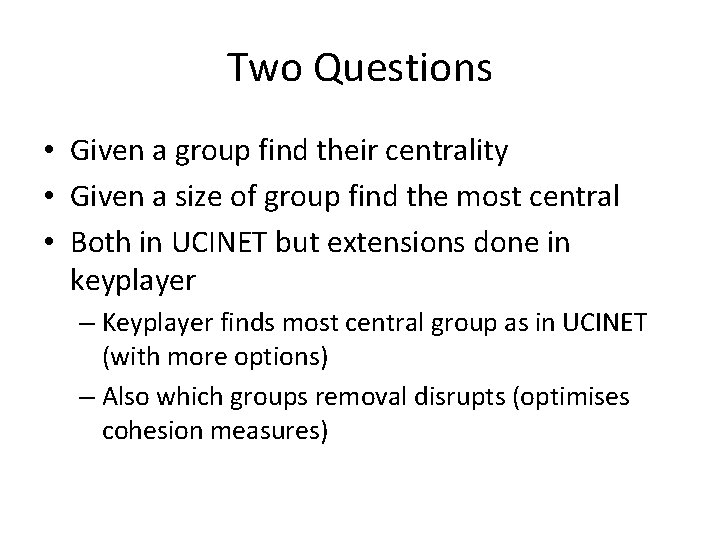
Two Questions • Given a group find their centrality • Given a size of group find the most central • Both in UCINET but extensions done in keyplayer – Keyplayer finds most central group as in UCINET (with more options) – Also which groups removal disrupts (optimises cohesion measures)

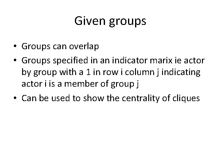
Given groups • Groups can overlap • Groups specified in an indicator marix ie actor by group with a 1 in row i column j indicating actor i is a member of group j • Can be used to show the centrality of cliques

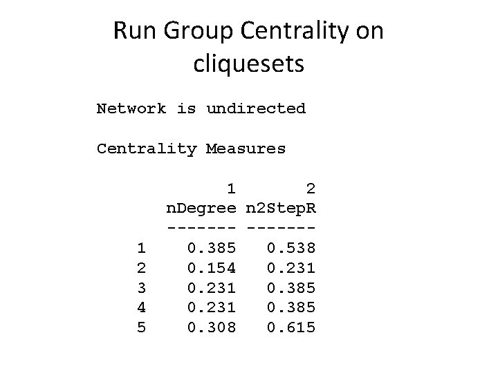
Padget Business 5 cliques found. • • • 1: 2: 3: 4: 5: BARBADORI GINORI MEDICI BISCHERI GUADAGNI LAMBERTES BISCHERI LAMBERTES PERUZZI CASTELLAN LAMBERTES PERUZZI BARBADORI CASTELLAN PERUZZI

Run Group Centrality on cliquesets Network is undirected Centrality Measures 1 2 3 4 5 1 2 n. Degree n 2 Step. R -------0. 385 0. 538 0. 154 0. 231 0. 385 0. 308 0. 615

Optimize using 3 actors

Flow betweenness • For valued data • Calculates flow between all pairs of actors – Delete actor recalculate – See how much flow has to go through actor • Example of an induced centrality using a network invariant

Network Invariants • An invariant is a measure that does not depend on the labels • Number of edges, number of actors, number of cycles of length four, network flow • Number of actors connected to Nick is not an invariant

Induced Centrality • An induced centrality is a centrality measure derived by measuring the contribution a node makes to an invariant. • Calculate the invariant, delete node, recalculate difference gives contribution • Could be done on edges as well as groups of actors

Simple Example • Graph invariant = number of edges Induced centrality = degree centrality • Can use any graph invariant and hence produce even more centrality measures

Centrality is itself an invariant Take any centrality measure Add all the scores together for a network This sum is an invariant Calculate the induced centrality measure of the centrality invariant. • Call this new centrality total centrality • •

Example Degree • Suppose an actor has degree x • Let the total degree be T • If I delete the actor then the total degree is equal to T-2 x • Total centrality is the actors centrality plus the centrality it gives to others

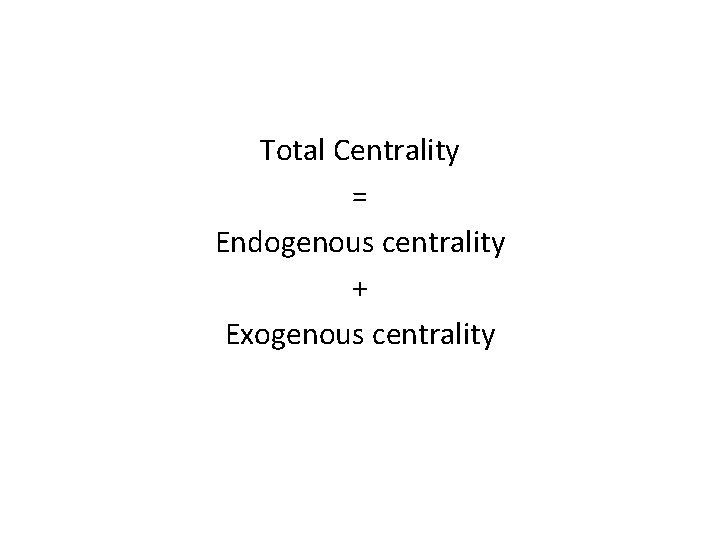
Exogenous centrality Take a centrality measure Calculate total centrality Total centrality – deleted actor centrality = How much centrality the deleted actor gives to others. Call this exogenous centrality and call the original centrality endogenous centrality

Total Centrality = Endogenous centrality + Exogenous centrality

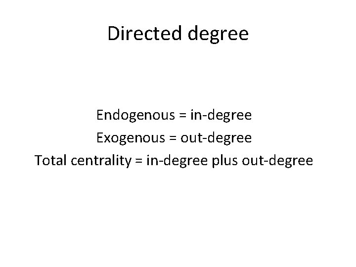
Directed degree Endogenous = in-degree Exogenous = out-degree Total centrality = in-degree plus out-degree

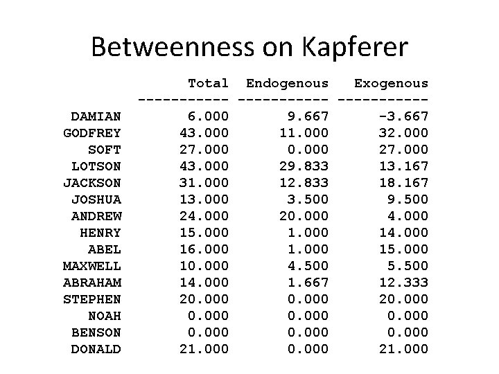
Betweenness on Kapferer DAMIAN GODFREY SOFT LOTSON JACKSON JOSHUA ANDREW HENRY ABEL MAXWELL ABRAHAM STEPHEN NOAH BENSON DONALD Total Endogenous Exogenous -----------6. 000 9. 667 -3. 667 43. 000 11. 000 32. 000 27. 000 0. 000 27. 000 43. 000 29. 833 13. 167 31. 000 12. 833 18. 167 13. 000 3. 500 9. 500 24. 000 20. 000 4. 000 15. 000 14. 000 16. 000 15. 000 10. 000 4. 500 5. 500 14. 000 1. 667 12. 333 20. 000 0. 000 21. 000

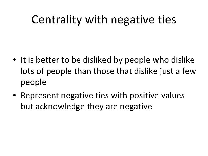
Centrality with negative ties • It is better to be disliked by people who dislike lots of people than those that dislike just a few people • Represent negative ties with positive values but acknowledge they are negative

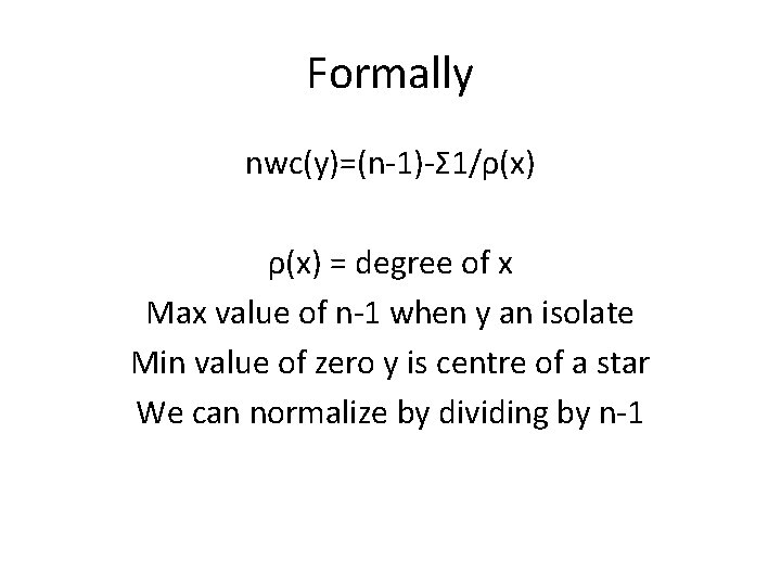
Formally nwc(y)=(n-1)-Σ 1/ρ(x) = degree of x Max value of n-1 when y an isolate Min value of zero y is centre of a star We can normalize by dividing by n-1

Directed data Dislike • In-degree = how much disliked amongst all other network members • Out-degree = emotional intenseness or possible aggression

Weighting • Receiving from high out-degree actor not as negative as from a low out-degree actor • Sending to a high in-degree actor not as negative as sending to a low in-degree actor

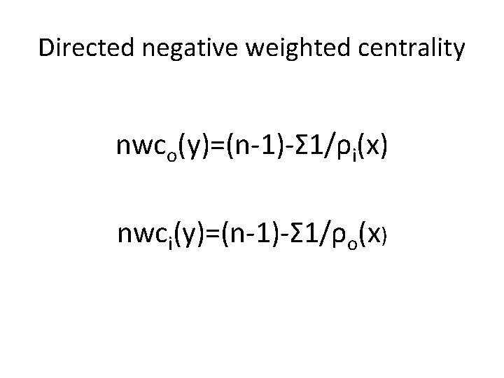
Directed negative weighted centrality nwco(y)=(n-1)-Σ 1/ρi(x) nwci(y)=(n-1)-Σ 1/ρo(x)

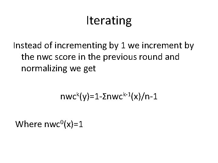
Iterating Instead of incrementing by 1 we increment by the nwc score in the previous round and normalizing we get nwck(y)=1 -Σnwck-1(x)/n-1 Where nwc 0(x)=1

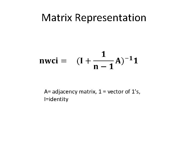
Matrix Representation A= adjacency matrix, 1 = vector of 1’s, I=identity

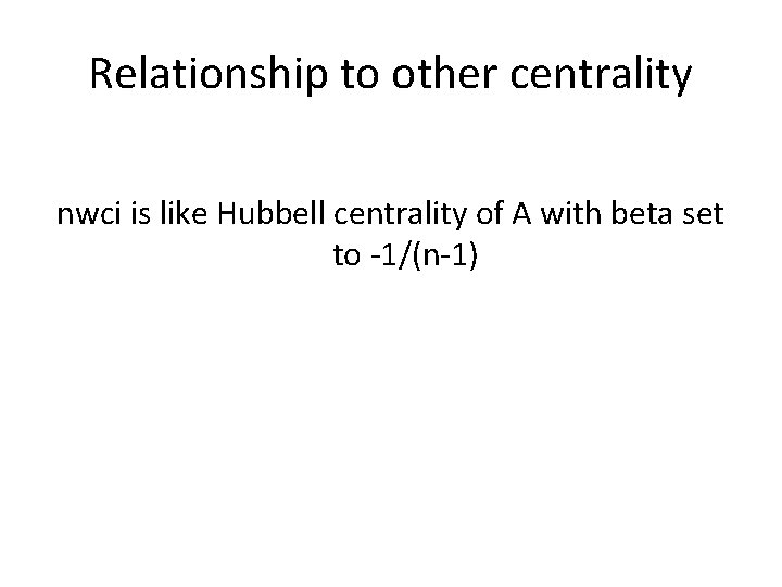
Relationship to other centrality nwci is like Hubbell centrality of A with beta set to -1/(n-1)

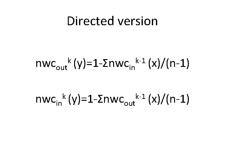
Directed version nwcoutk (y)=1 -Σnwcink-1 (x)/(n-1) nwcink (y)=1 -Σnwcoutk-1 (x)/(n-1)

Matrix Formulations

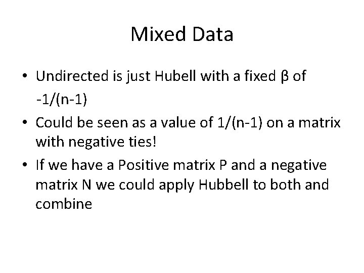
Mixed Data • Undirected is just Hubell with a fixed β of -1/(n-1) • Could be seen as a value of 1/(n-1) on a matrix with negative ties! • If we have a Positive matrix P and a negative matrix N we could apply Hubbell to both and combine

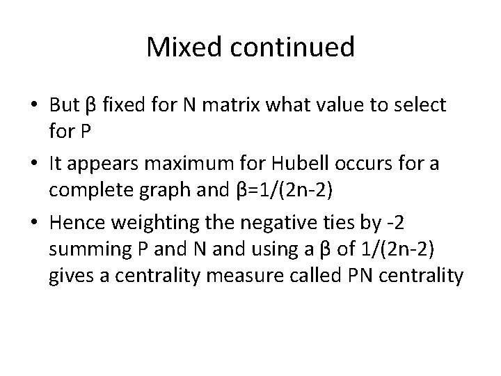
Mixed continued • But β fixed for N matrix what value to select for P • It appears maximum for Hubell occurs for a complete graph and β=1/(2 n-2) • Hence weighting the negative ties by -2 summing P and N and using a β of 1/(2 n-2) gives a centrality measure called PN centrality

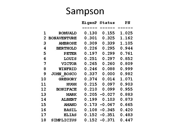
Sampson 1 ROMUALD 2 BONAVENTURE 3 AMBROSE 4 BERTHOLD 5 PETER 6 LOUIS 7 VICTOR 8 WINFRID 9 JOHN_BOSCO 10 GREGORY 11 HUGH 12 BONIFACE 13 MARK 14 ALBERT 15 AMAND 16 BASIL 17 ELIAS 18 SIMPLICIUS Eigen. P -----0. 130 0. 301 0. 309 0. 226 0. 197 0. 251 0. 265 0. 246 0. 337 0. 374 0. 215 0. 210 0. 205 0. 199 0. 173 0. 108 0. 152 Status PN ------0. 155 1. 025 0. 325 1. 162 0. 339 1. 105 0. 295 0. 944 0. 299 0. 761 0. 297 0. 852 0. 260 0. 809 0. 088 0. 999 0. 000 0. 982 0. 014 1. 071 0. 097 0. 903 0. 099 0. 955 -0. 027 0. 883 0. 103 0. 873 -0. 067 0. 665 -0. 345 0. 420 -0. 351 0. 483 -0. 371 0. 447