Central Limit Theorem ANOVA ANOVA ANOVA Total Sum


 Σύνολο 1230 (1238) 1255 Όχι κάπνισμα")


 (y - my)")
 covariance = ∑(x - mx)(y - my)/(n-1) (y - my)")
 correlation = ∑(x - mx)(y - my) √(∑(x - m")


 60")


- Slides: 49
Central Limit Theorem Κανονική κατανομή
ANOVA
ANOVA
ANOVA Total Sum of Squares Within Group SS Between Group SS
DF SS Mean S F MST / MSE Between Groups g-1 SST / df Within Groups n-g SSE / df Total n-1 Total Sum of Squares Within Group SS Between Group SS
Μη παραμετρικές μέθοδοι • • • t-test Paired t-test ANOVA Two way ANOVA Pearson’s correlation • • • Mann Whitney U-test Wilcoxon’s signed ranks test Kruskal-Wallis Friedman Spearman’s rank correlation
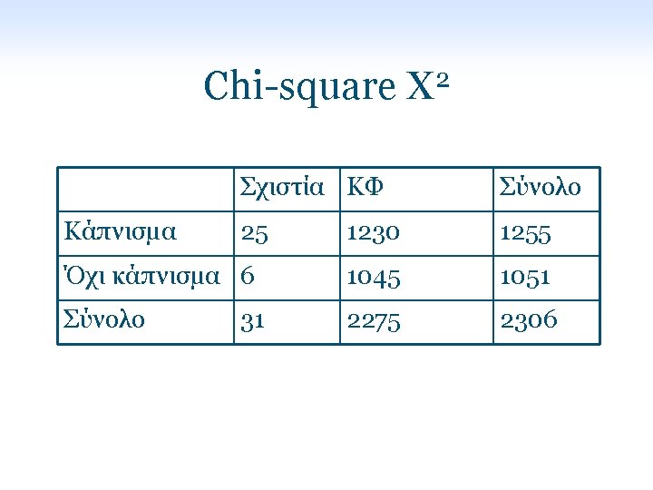
Chi-square X 2 Σχιστία ΚΦ Κάπνισμα 25 (17) Σύνολο 1230 (1238) 1255 Όχι κάπνισμα 6 (14) 1045 (1037) 1051 Σύνολο 2275 31 X 2 = ∑ [(O – E) 2 / E] = 8. 7 P = 0. 0032 2306
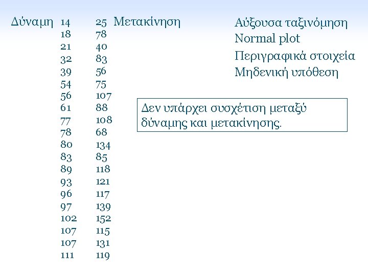
Δύναμη 78 107 21 18 96 89 93 32 77 102 56 80 54 61 111 97 14 39 83 68 Μετακίνηση 131 40 78 117 118 121 83 108 115 152 107 134 75 88 119 139 25 56 85
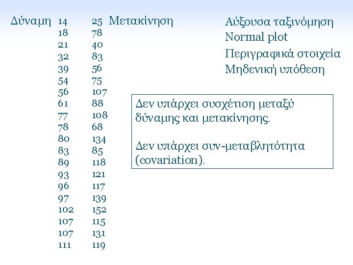
Δύναμη 14 18 21 32 39 54 56 61 77 78 80 83 89 93 96 97 102 107 111 25 Μετακίνηση 78 40 83 56 75 107 88 108 68 134 85 118 121 117 139 152 115 131 119 Αύξουσα ταξινόμηση
Δύναμη 14 18 21 32 39 54 56 61 77 78 80 83 89 93 96 97 102 107 111 25 Μετακίνηση 78 40 83 56 75 107 88 108 68 134 85 118 121 117 139 152 115 131 119 Αύξουσα ταξινόμηση Normal plot 2 1 0 -1 -2 0 30 60 90 120 X
Δύναμη 14 18 21 32 39 54 56 61 77 78 80 83 89 93 96 97 102 107 111 25 Μετακίνηση 78 40 83 56 75 107 88 108 68 134 85 118 121 117 139 152 115 131 119 Αύξουσα ταξινόμηση Normal plot 2 1 0 -1 -2 10 60 110 160 Y
Δύναμη 14 18 21 32 39 54 56 61 77 78 80 83 89 93 96 97 102 107 111 25 Μετακίνηση 78 40 83 56 75 107 88 Mean 108 Variance 68 Std. Deviation 134 Minimum 85 Maximum 118 121 Median 117 139 152 115 131 119 Αύξουσα ταξινόμηση Normal plot Περιγραφικά στοιχεία 70. 7 1015. 14 31. 86 14 111 79. 0 97. 9 1155. 94 33. 99 25 152 107. 5
Δύναμη 14 18 21 32 39 54 56 61 77 78 80 83 89 93 96 97 102 107 111 25 Μετακίνηση 78 40 83 56 75 107 88 Mean 108 Variance 68 Std. Deviation 134 Minimum 85 Maximum 118 121 Median 117 139 152 115 131 119 Αύξουσα ταξινόμηση Normal plot Περιγραφικά στοιχεία Μηδενική υπόθεση 70. 7 1015. 14 31. 86 14 111 79. 0 97. 9 1155. 94 33. 99 25 152 107. 5
Covariation
Covariation
Covariation (x - mx) (y - my)
Covariation (x - mx) covariance = ∑(x - mx)(y - my)/(n-1) (y - my) variance = ∑(x - mx)2/(n-1)
Covariation (x - mx) correlation = ∑(x - mx)(y - my) √(∑(x - m ) ∑(y - m ) ) x (y - my) 2 y 2
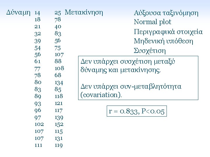
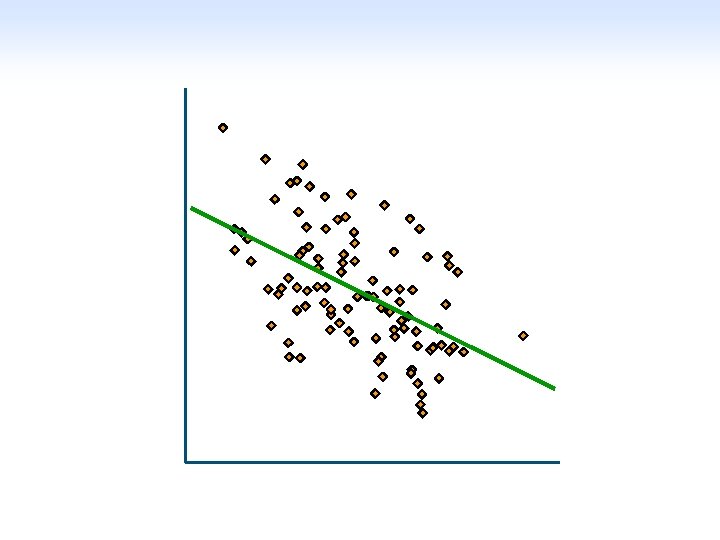
Δύναμη 14 18 21 32 39 54 56 61 77 78 80 83 89 93 96 97 102 107 111 25 Μετακίνηση Αύξουσα ταξινόμηση 78 Normal plot 40 Περιγραφικά στοιχεία 83 56 Μηδενική υπόθεση 75 Συσχέτιση 107 88 108 Correlation coefficient (Pearson’s): 68 134 r = 0. 833, P<0. 05 85 118 Coefficient of determination: 121 2 = 0. 694 = 69. 4% r 117 139 152 115 131 119
160 140 dependent 120 100 80 60 40 20 0 0 20 40 60 independent 80 100 120
160 140 dependent 120 100 80 60 40 20 0 0 20 40 60 independent 80 100 120
160 140 dependent residual 120 100 80 60 40 20 0 0 20 40 60 independent 80 100 120
160 140 dependent 120 100 80 60 40 20 0 0 20 40 60 independent 80 100 120
160 140 dependent 120 y = ax + b 100 80 slope (κλίση) 60 intercept 40 20 0 0 20 40 60 independent 80 100 120
160 140 dependent 120 100 80 60 40 20 0 0 20 40 60 independent 80 100 120
80 y = 1 x + 0 70 60 50 40 30 20 10 0 0 10 20 30 40 50 60 70 80
80 70 60 50 40 30 20 10 0 0 10 20 30 40 50 60 70 80
80 y = 0. 8421 x + 6. 3158 70 60 50 40 30 20 10 0 0 10 20 30 40 50 60 70 80
160 95% prediction interval 140 122 120 100 80 80 60 40 38 20 0 0 20 40 60 80 100 120
450 400 350 300 y = 0. 7378 x + 29. 576 R 2 = 0. 4642 250 200 150 100 50 0 0 50 100 150 200 250 300 350 400
250 y = 1. 4893 x + 50. 654 R 2 = 0. 9945 200 150 100 ς α τ τη ό σ ι ή μ μ α Γρ 50 0 0 20 40 60 80 100 120
Χ Υ Χ-Υ 100 80 y = 0. 9088 x - 76. 281 R 2 = 0. 4142 60 40 20 0 0 -20 -40 -60 -80 20 40 60 80 100 120 140 160
d 1 d 2
Πηγές και στατιστικά πακέτα • Γενικές σελίδες – http: //statpages. org/ – http: //www. freestatistics. info/index. php • Λογισμικό – SPSS, SAS, … – www. socr. ucla. edu Java λογισμικό (online), ελεύθερο – http: //folk. uio. no/ohammer/past/ – www. statsdirect. com Απλό, με καλό αρχείο βοήθειας (£ 99) • Υπολογισμός μεγέθους δείγματος – http: //biostat. mc. vanderbilt. edu/twiki/bin/view/Main/Power. Sam ple. Size – http: //www. stat. uiowa. edu/~rlenth/Power/index. html
Ασκήσεις • Angle Orthod 2010; 80: 435 -439 • Angle Orthod 2010; 80: 254– 261