Center Computational CCV Visualization Mannheim Summer School 2002

Center Computational CCV Visualization Mannheim Summer School 2002 Computational Visualization 1. Sources, characteristics, representation 2. Mesh Processing 3. Contouring 4. Volume Rendering 5. Flow, Vector, Tensor Field Visualization 6. Application Case Studies Copyright: Chandrajit Bajaj, CCV, University of Texas at Austin

Center Computational CCV Visualization Computational Visualization: sources, characteristics and representation Lecture 1 Copyright: Chandrajit Bajaj, CCV, University of Texas at Austin

Center Computational CCV Outline Visualization • • Data Sources: Meshless and Meshed Mesh and Field Data Characteristics Mesh Representations Mesh Finite Elements Copyright: Chandrajit Bajaj, CCV, University of Texas at Austin

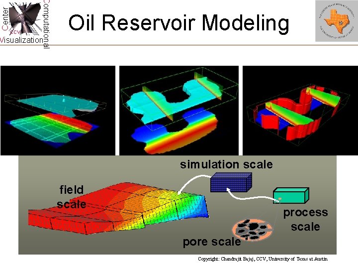
Center Computational CCV Oil Reservoir Modeling Visualization Multi-scale Oil Reservoir Modeling, Simulation, and Visualization simulation scale field scale rf process scale pore scale Copyright: Chandrajit Bajaj, CCV, University of Texas at Austin

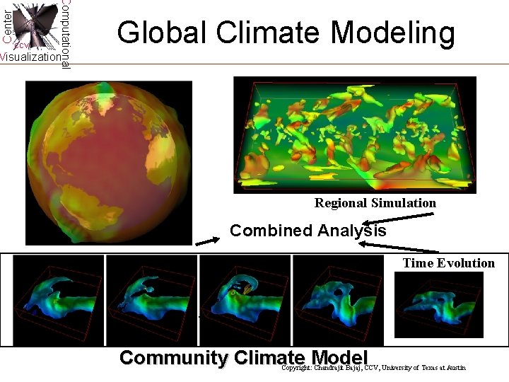
Center Computational CCV Global Climate Modeling Visualization Regional Simulation Global Simulation Combined Analysis Time Evolution Community Climate Model Copyright: Chandrajit Bajaj, CCV, University of Texas at Austin

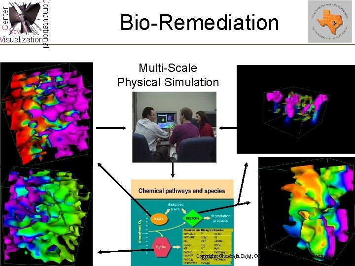
Center Computational CCV Bio-Remediation Visualization Multi-Scale Physical Simulation Study of pollutant diffusion over the years Copyright: Chandrajit Bajaj, CCV, University of Texas at Austin

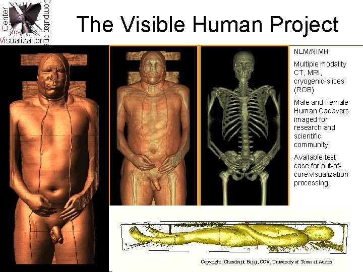
Center Computational CCV Visualization The Visible Human Project NLM/NIMH Multiple modality CT, MRI, cryogenic-slices (RGB) Male and Female Human Cadavers imaged for research and scientific community Available test case for out-ofcore visualization processing Copyright: Chandrajit Bajaj, CCV, University of Texas at Austin

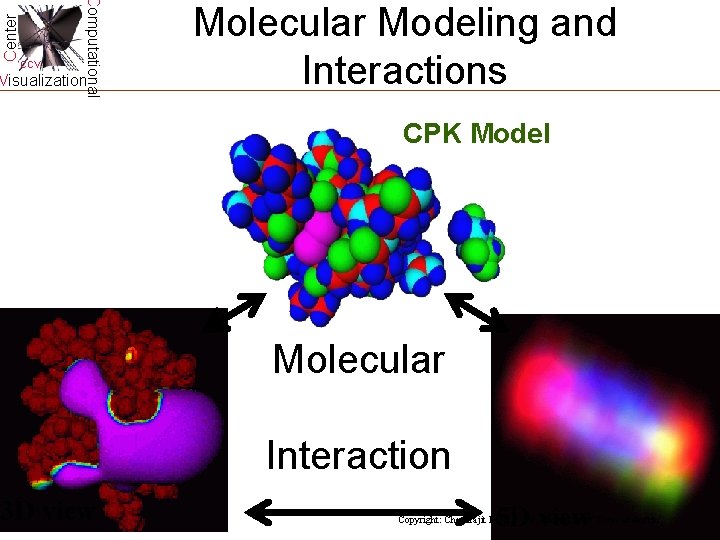
Center Computational CCV Visualization Molecular Modeling and Interactions CPK Model Molecular Interaction 3 D view 5 D view Copyright: Chandrajit Bajaj, CCV, University of Texas at Austin

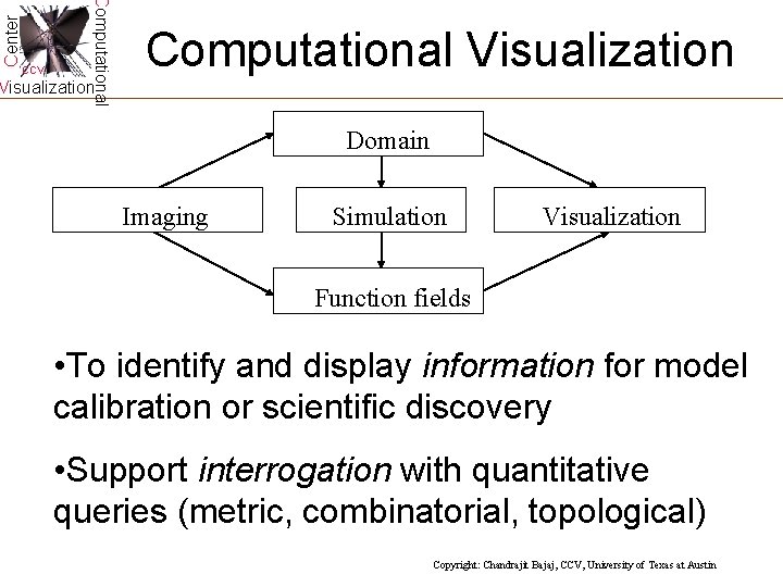
Center Computational CCV Computational Visualization Domain Imaging Simulation Visualization Function fields • To identify and display information for model calibration or scientific discovery • Support interrogation with quantitative queries (metric, combinatorial, topological) Copyright: Chandrajit Bajaj, CCV, University of Texas at Austin

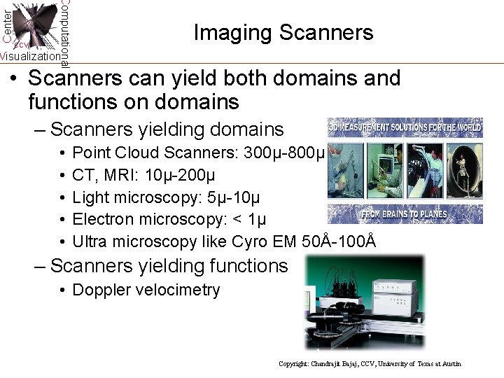
Center Computational CCV Imaging Scanners Visualization • Scanners can yield both domains and functions on domains – Scanners yielding domains • • • Point Cloud Scanners: 300μ-800μ CT, MRI: 10μ-200μ Light microscopy: 5μ-10μ Electron microscopy: < 1μ Ultra microscopy like Cyro EM 50Å-100Å – Scanners yielding functions • Doppler velocimetry Copyright: Chandrajit Bajaj, CCV, University of Texas at Austin

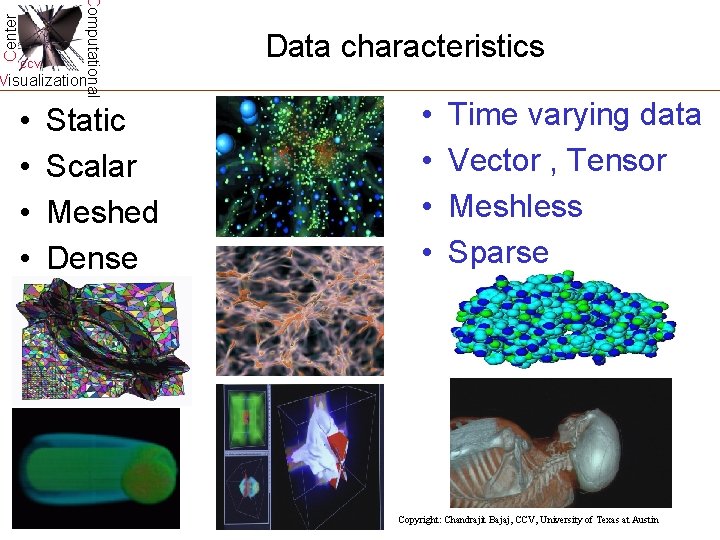
Center Computational CCV Data characteristics Visualization • • Static Scalar Meshed Dense • • Time varying data Vector , Tensor Meshless Sparse Copyright: Chandrajit Bajaj, CCV, University of Texas at Austin

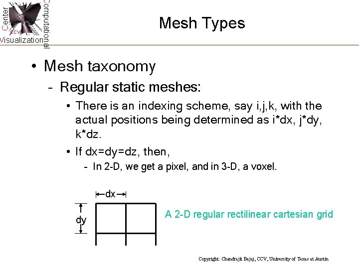
Center Computational CCV Mesh Types Visualization • Mesh taxonomy – Regular static meshes: • There is an indexing scheme, say i, j, k, with the actual positions being determined as i*dx, j*dy, k*dz. • If dx=dy=dz, then, – In 2 -D, we get a pixel, and in 3 -D, a voxel. dx dy A 2 -D regular rectilinear cartesian grid Copyright: Chandrajit Bajaj, CCV, University of Texas at Austin

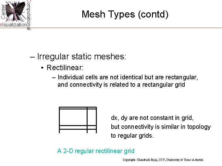
Center Computational CCV Mesh Types (contd) Visualization – Irregular static meshes: • Rectilinear: – Individual cells are not identical but are rectangular, and connectivity is related to a rectangular grid dx, dy are not constant in grid, but connectivity is similar in topology to regular grids. A 2 -D regular rectilinear grid Copyright: Chandrajit Bajaj, CCV, University of Texas at Austin

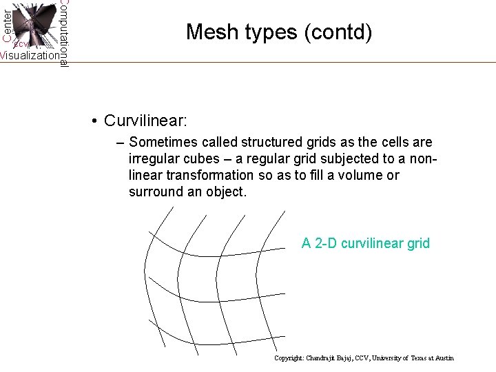
Center Computational CCV Mesh types (contd) Visualization • Curvilinear: – Sometimes called structured grids as the cells are irregular cubes – a regular grid subjected to a nonlinear transformation so as to fill a volume or surround an object. A 2 -D curvilinear grid Copyright: Chandrajit Bajaj, CCV, University of Texas at Austin

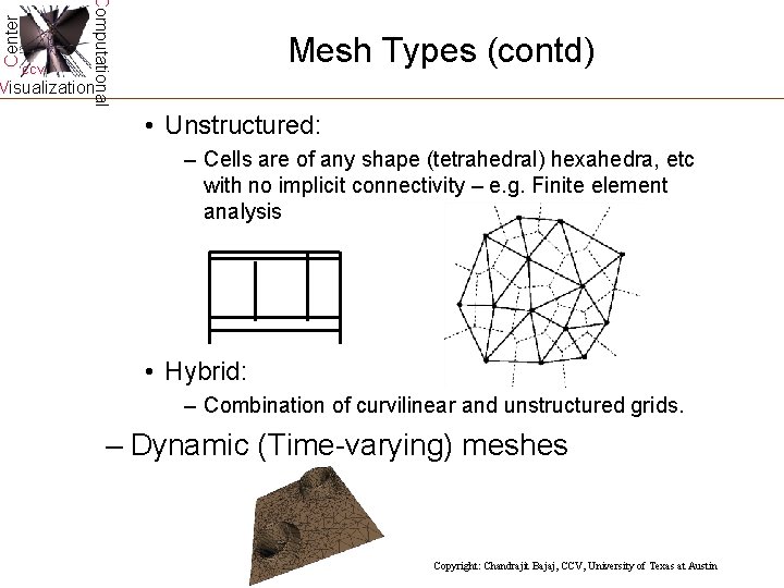
Center Computational CCV Mesh Types (contd) Visualization • Unstructured: – Cells are of any shape (tetrahedral) hexahedra, etc with no implicit connectivity – e. g. Finite element analysis • Hybrid: – Combination of curvilinear and unstructured grids. – Dynamic (Time-varying) meshes Copyright: Chandrajit Bajaj, CCV, University of Texas at Austin

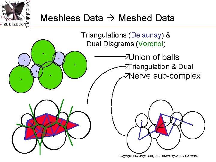
Center Computational CCV Visualization Meshless Data Meshed Data Triangulations (Delaunay) & Dual Diagrams (Voronoi) äUnion of balls äTriangulation & Dual äNerve sub-complex Copyright: Chandrajit Bajaj, CCV, University of Texas at Austin

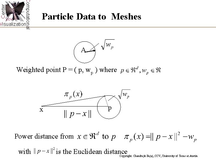
Center Computational CCV Particle Data to Meshes Visualization A Weighted point P = ( p, wp ) where p x Power distance from with is the Euclidean distance Copyright: Chandrajit Bajaj, CCV, University of Texas at Austin

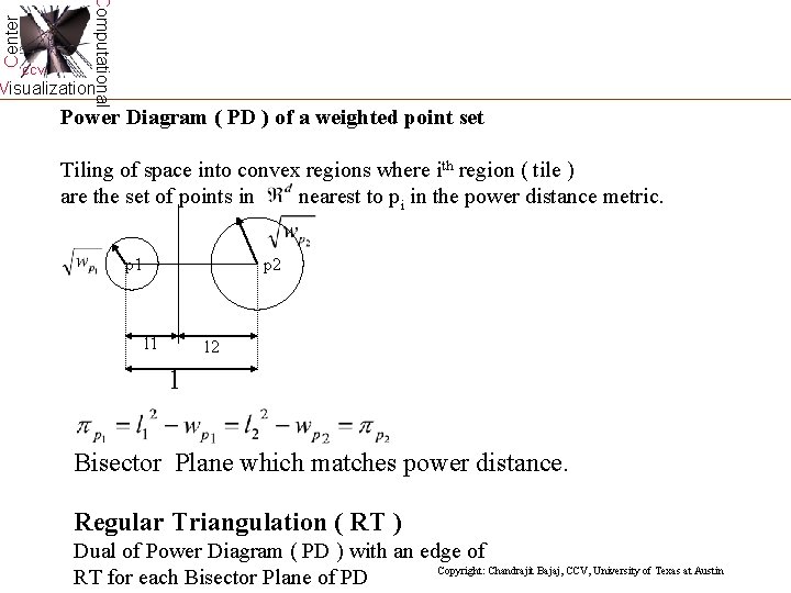
Center Computational CCV Visualization Power Diagram ( PD ) of a weighted point set Tiling of space into convex regions where ith region ( tile ) are the set of points in nearest to pi in the power distance metric. p 1 p 2 l 1 l 2 l Bisector Plane which matches power distance. Regular Triangulation ( RT ) Dual of Power Diagram ( PD ) with an edge of Copyright: Chandrajit Bajaj, CCV, University of Texas at Austin RT for each Bisector Plane of PD

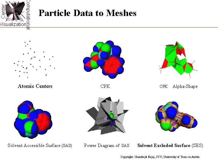
Center Computational CCV Particle Data to Meshes Visualization Atomic Centers Solvent Accessible Surface (SAS) CPK Power Diagram of SAS Alpha-Shape Solvent Excluded Surface (SES) Copyright: Chandrajit Bajaj, CCV, University of Texas at Austin

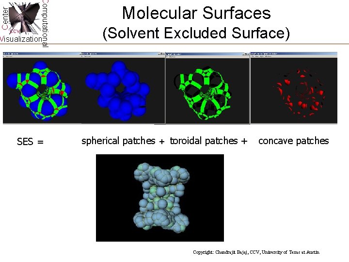
Center Computational CCV Visualization SES = Molecular Surfaces (Solvent Excluded Surface) spherical patches + toroidal patches + concave patches Copyright: Chandrajit Bajaj, CCV, University of Texas at Austin

Center Computational CCV Field Data Visualization • Scalar temperature, pressure, density, energy, change, resistance, capacitance, refractive index, wavelength, frequency & fluid content. • Vector velocity, acceleration, angular velocity, force, momentum, magnetic field, electric field, gravitational field, current, surface normal • Tensor stress, strain, conductivity, moment of inertia and electromagnetic field • Multivariate Time Series Copyright: Chandrajit Bajaj, CCV, University of Texas at Austin

Center Computational CCV Field Data on Meshes Visualization • Finite elements commonly used – Linear finite elements – Non-linear finite elements • Interpolants/Approximants used to approximate the data on the domain (Lagrange, Hermite, …) Copyright: Chandrajit Bajaj, CCV, University of Texas at Austin

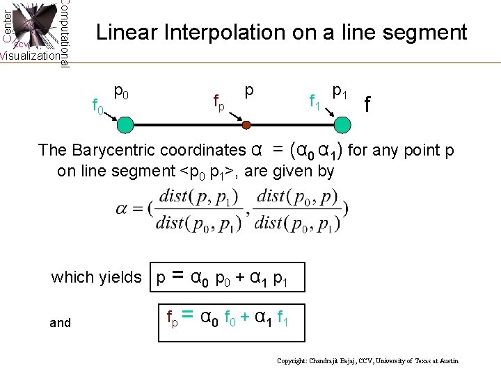
Center Computational CCV Linear Interpolation on a line segment Visualization p 0 f 0 p 1 fp f 1 f The Barycentric coordinates α = (α 0 α 1) for any point p on line segment <p 0 p 1>, are given by which yields p = α 0 p 0 + α 1 p 1 and fp = α 0 f 0 + α 1 f 1 Copyright: Chandrajit Bajaj, CCV, University of Texas at Austin

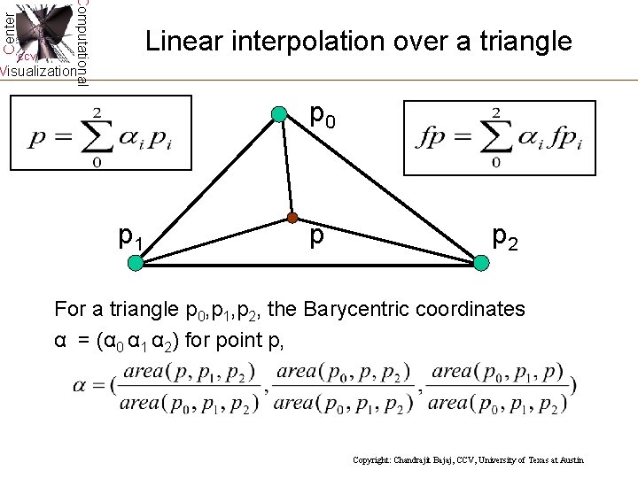
Center Computational CCV Linear interpolation over a triangle Visualization p 0 p 1 p p 2 For a triangle p 0, p 1, p 2, the Barycentric coordinates α = (α 0 α 1 α 2) for point p, Copyright: Chandrajit Bajaj, CCV, University of Texas at Austin

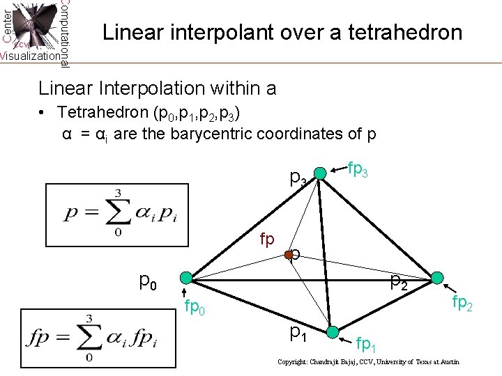
Center Computational CCV Linear interpolant over a tetrahedron Visualization Linear Interpolation within a • Tetrahedron (p 0, p 1, p 2, p 3) α = αi are the barycentric coordinates of p p 3 fp fp 3 p p 0 p 2 fp 0 p 1 fp 2 fp 1 Copyright: Chandrajit Bajaj, CCV, University of Texas at Austin

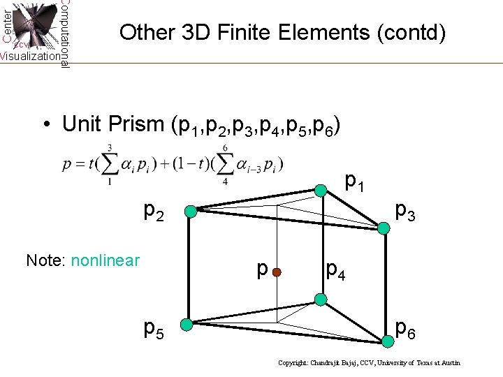
Center Computational CCV Other 3 D Finite Elements (contd) Visualization • Unit Prism (p 1, p 2, p 3, p 4, p 5, p 6) p 1 p 2 Note: nonlinear p 3 p p 5 p 4 p 6 Copyright: Chandrajit Bajaj, CCV, University of Texas at Austin

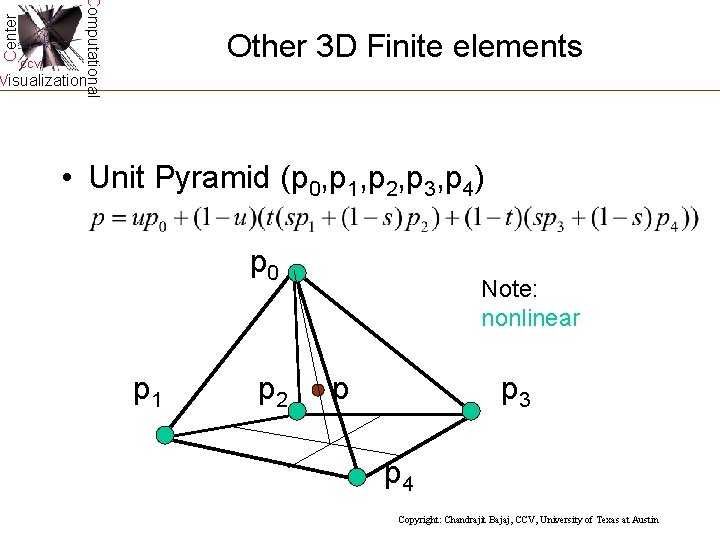
Center Computational CCV Other 3 D Finite elements Visualization • Unit Pyramid (p 0, p 1, p 2, p 3, p 4) p 0 p 1 Note: nonlinear p 2 p p 3 p 4 Copyright: Chandrajit Bajaj, CCV, University of Texas at Austin

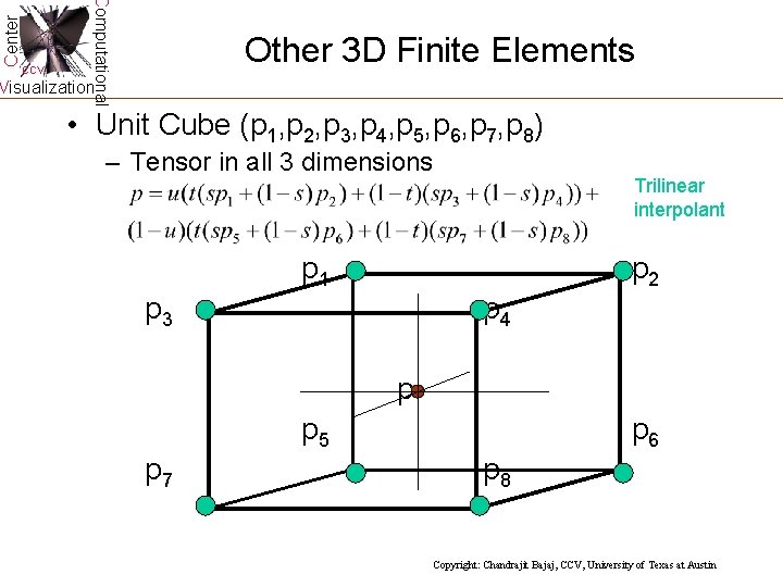
Center Computational CCV Other 3 D Finite Elements Visualization • Unit Cube (p 1, p 2, p 3, p 4, p 5, p 6, p 7, p 8) – Tensor in all 3 dimensions Trilinear interpolant p 1 p 2 p 3 p 4 p p 5 p 7 p 6 p 8 Copyright: Chandrajit Bajaj, CCV, University of Texas at Austin

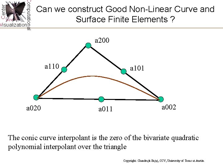
Center Computational CCV Visualization Can we construct Good Non-Linear Curve and Surface Finite Elements ? a 200 a 110 a 020 a 101 a 011 a 002 The conic curve interpolant is the zero of the bivariate quadratic polynomial interpolant over the triangle Copyright: Chandrajit Bajaj, CCV, University of Texas at Austin

Center Computational CCV Visualization Every good answer needs coffee! Or Mineralwasser !! Copyright: Chandrajit Bajaj, CCV, University of Texas at Austin

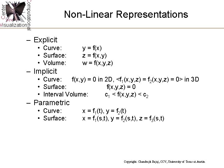
Center Computational CCV Non-Linear Representations Visualization – Explicit • Curve: • Surface: • Volume: y = f(x) z = f(x, y) w = f(x, y, z) – Implicit • Curve: f(x, y) = 0 in 2 D, <f 1(x, y, z) = f 2(x, y, z) = 0> in 3 D • Surface: f(x, y, z) = 0 • Interval Volume: c 1 < f(x, y, z) < c 2 – Parametric • Curve: • Surface: x = f 1(t), y = f 2(t) x = f 1(s, t), y = f 2(s, t), z = f 3(s, t) Copyright: Chandrajit Bajaj, CCV, University of Texas at Austin

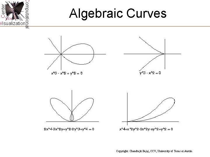
Center Computational CCV Algebraic Curves Visualization Copyright: Chandrajit Bajaj, CCV, University of Texas at Austin

Center Computational CCV Implict vs Parametric Visualization • Curves • Surfaces • Volumes Copyright: Chandrajit Bajaj, CCV, University of Texas at Austin

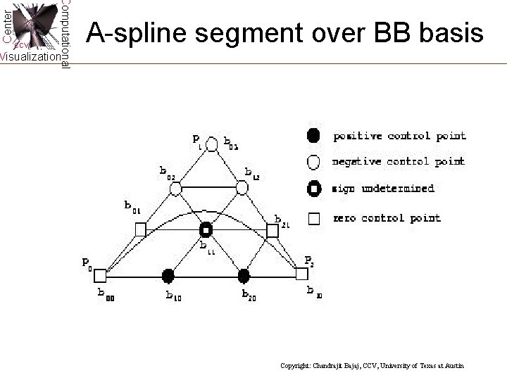
Center Computational CCV A-spline segment over BB basis Visualization Copyright: Chandrajit Bajaj, CCV, University of Texas at Austin

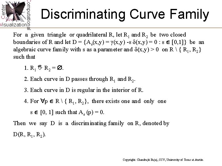
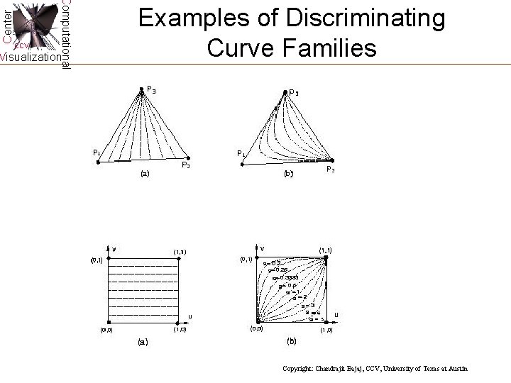
Center Computational CCV Discriminating Curve Family Visualization For a given triangle or quadrilateral R, let R 1 and R 2 be two closed boundaries of R and let D = {As(x, y) = (x, y) -s (x, y) = 0 : s [0, 1]} be an algebraic curve family with s as a parameter and (x, y) > 0 on R { R 1, R 2} such that 1. R 1 R 2 = . 2. Each curve in D passes through R 1 and R 2. 3. Each curve in D is regular in the interior of R. 4. For p R { R 1, R 2}, there exists one and only one s [0, 1] such that As (p) = 0. Then we say D is a discriminating family on R, denoted by D(R, R 1, R 2). Copyright: Chandrajit Bajaj, CCV, University of Texas at Austin

Center Computational CCV Visualization Examples of Discriminating Curve Families Copyright: Chandrajit Bajaj, CCV, University of Texas at Austin

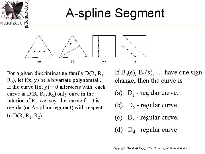
Center Computational CCV A-spline Segment Visualization For a given discriminating family D(R, R 1, R 2), let f(x, y) be a bivariate polynomial. If the curve f(x, y) = 0 intersects with each curve in D(R, R 1, R 2) only once in the interior of R, we say the curve f = 0 is regular(or A-spline segment) with respect to D(R, R 1, R 2). If B 0(s), B 1(s), … have one sign change, then the curve is (a) D 1 - regular curve. (b) D 2 - regular curve. (c) D 3 - regular curve. (d) D 4 - regular curve. Copyright: Chandrajit Bajaj, CCV, University of Texas at Austin

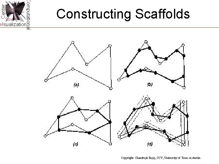
Center Computational CCV Constructing Scaffolds Visualization Copyright: Chandrajit Bajaj, CCV, University of Texas at Austin

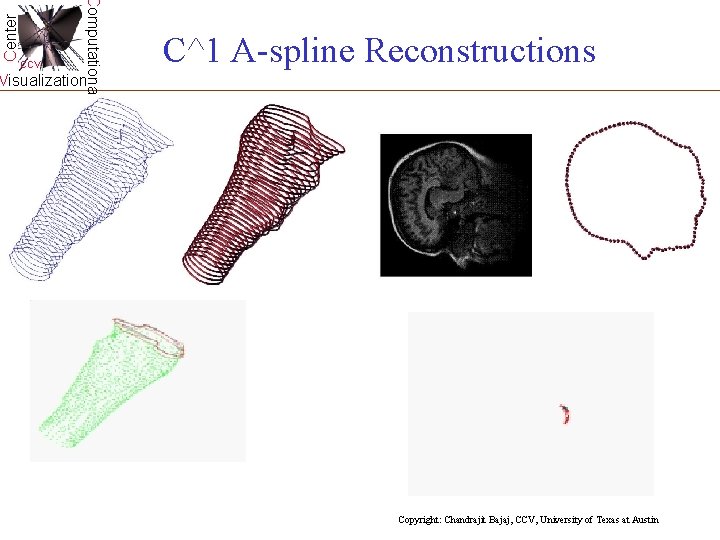
Center Computational CCV C^1 A-spline Reconstructions: Visualization Input contours G 1 / D 4 curves G 2 / D 4 curves Copyright: Chandrajit Bajaj, CCV, University of Texas at Austin

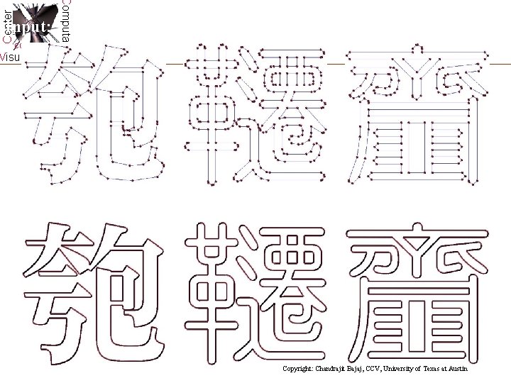
Center CCV Computational Input: Visualization G 1 / D 4 curves: Copyright: Chandrajit Bajaj, CCV, University of Texas at Austin

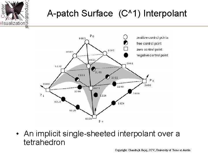
Center Computational CCV A-patch Surface (C^1) Interpolant Visualization • An implicit single-sheeted interpolant over a tetrahedron Copyright: Chandrajit Bajaj, CCV, University of Texas at Austin

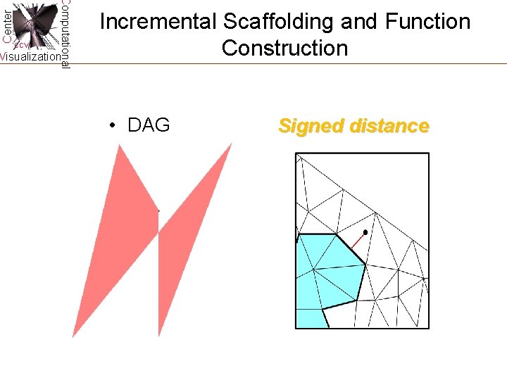
Center Computational CCV Visualization Incremental Scaffolding and Function Construction • DAG Signed distance

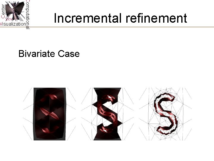
Center Computational CCV Visualization Incremental refinement Bivariate Case

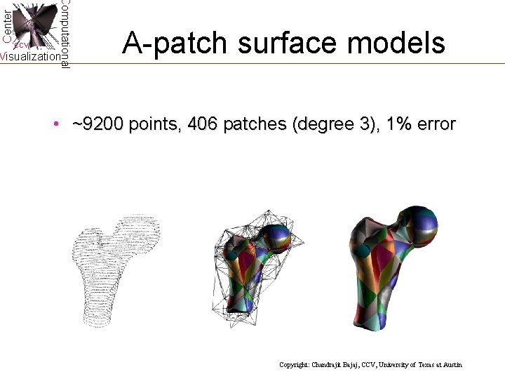
Center Computational CCV Visualization A-patch surface models • ~9200 points, 406 patches (degree 3), 1% error Copyright: Chandrajit Bajaj, CCV, University of Texas at Austin

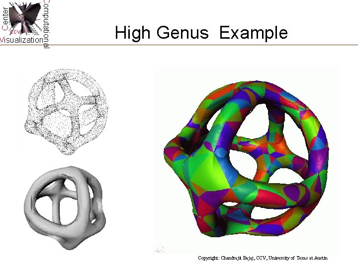
Center Computational CCV Visualization High Genus Example Copyright: Chandrajit Bajaj, CCV, University of Texas at Austin

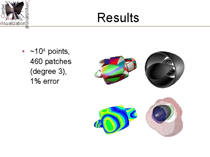
Center Computational CCV Visualization • ~104 points, 460 patches (degree 3), 1% error Results

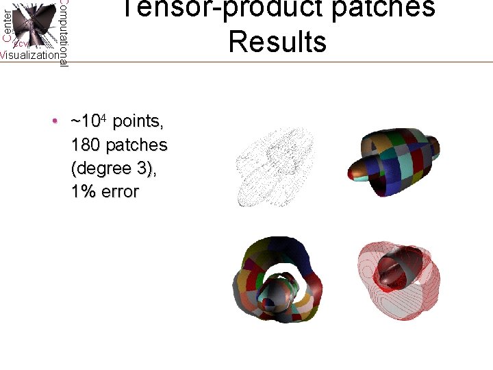
Center Computational CCV Visualization Tensor-product patches Results • ~104 points, 180 patches (degree 3), 1% error

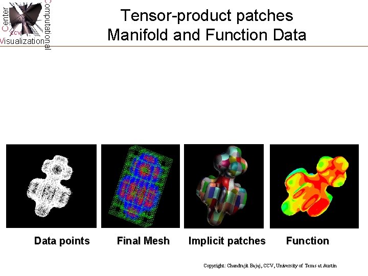
Center Computational CCV Visualization Data points Tensor-product patches Manifold and Function Data Final Mesh Implicit patches Function Copyright: Chandrajit Bajaj, CCV, University of Texas at Austin

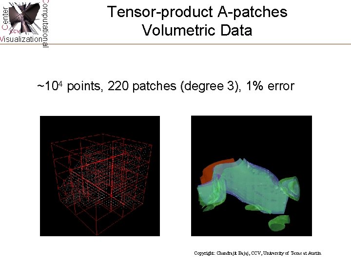
Center Computational CCV Visualization Tensor-product A-patches Volumetric Data ~104 points, 220 patches (degree 3), 1% error Copyright: Chandrajit Bajaj, CCV, University of Texas at Austin

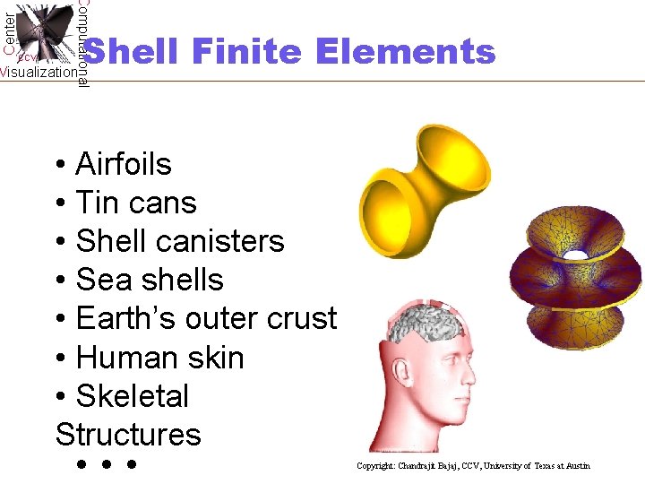
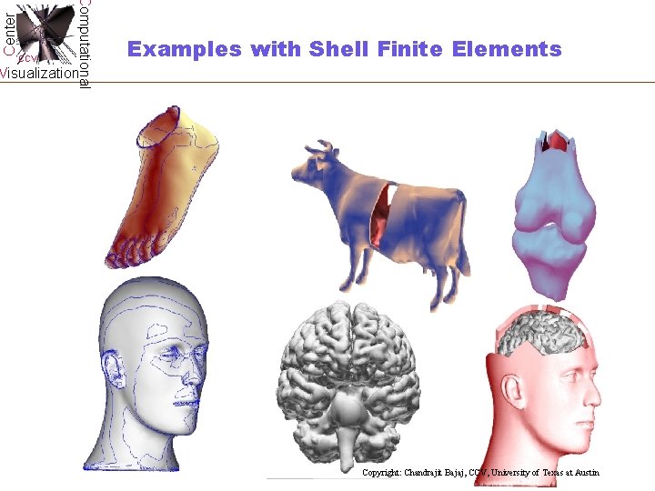
Center Computational CCV Visualization Shell Finite Elements • Airfoils • Tin cans • Shell canisters • Sea shells • Earth’s outer crust • Human skin • Skeletal Structures Copyright: Chandrajit Bajaj, CCV, University of Texas at Austin

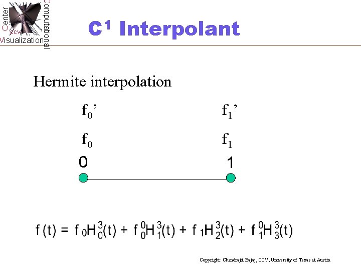
Center Computational CCV Visualization C 1 Interpolant Hermite interpolation f 0’ f 1’ f 0 0 f 1 1 Copyright: Chandrajit Bajaj, CCV, University of Texas at Austin

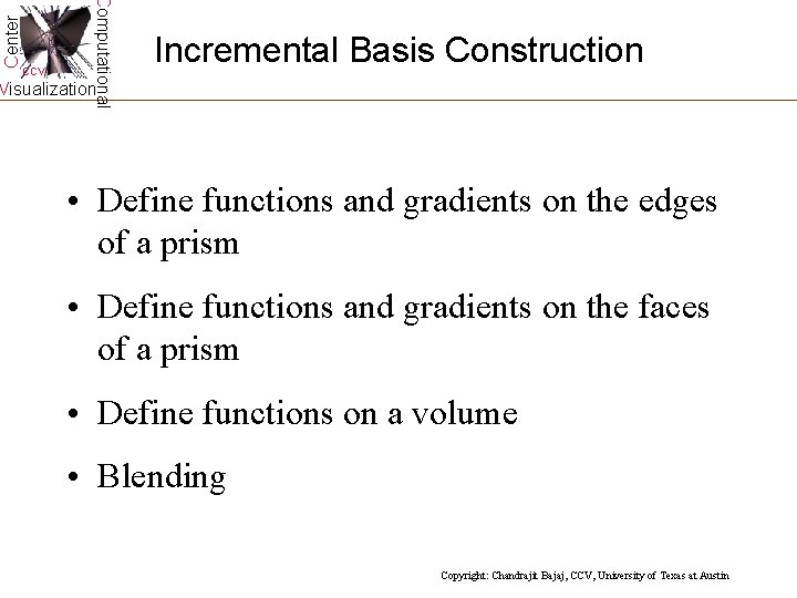
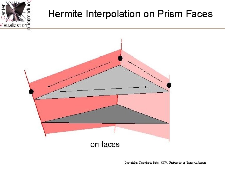
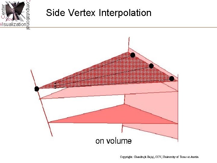
Center Computational CCV Incremental Basis Construction Visualization • Define functions and gradients on the edges of a prism • Define functions and gradients on the faces of a prism • Define functions on a volume • Blending Copyright: Chandrajit Bajaj, CCV, University of Texas at Austin

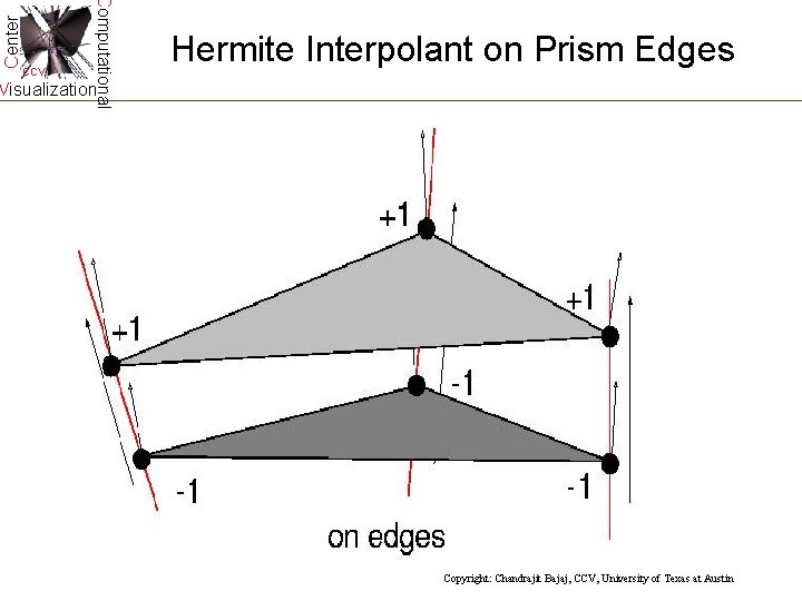
Center Computational CCV Hermite Interpolant on Prism Edges Visualization Copyright: Chandrajit Bajaj, CCV, University of Texas at Austin

Center Computational CCV Hermite Interpolation on Prism Faces Visualization Copyright: Chandrajit Bajaj, CCV, University of Texas at Austin

Center Computational CCV Side Vertex Interpolation Visualization Copyright: Chandrajit Bajaj, CCV, University of Texas at Austin

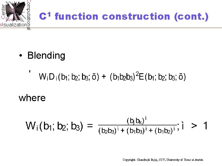
Center Computational CCV Visualization C 1 function construction (cont. ) • Blending where Copyright: Chandrajit Bajaj, CCV, University of Texas at Austin

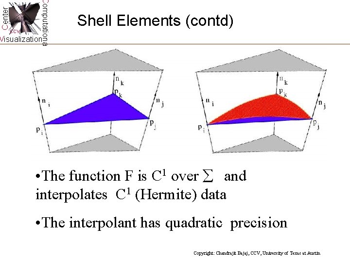
Center Computational CCV Shell Elements (contd) Visualization • The function F is C 1 over and interpolates C 1 (Hermite) data • The interpolant has quadratic precision Copyright: Chandrajit Bajaj, CCV, University of Texas at Austin

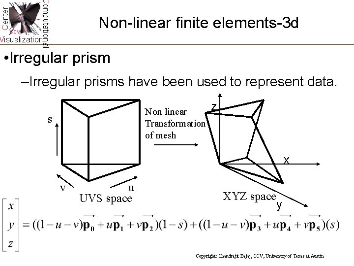
Center Computational CCV Non-linear finite elements-3 d Visualization • Irregular prism –Irregular prisms have been used to represent data. Non linear Transformation of mesh s z x v u UVS space XYZ space y Copyright: Chandrajit Bajaj, CCV, University of Texas at Austin

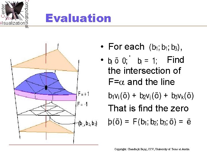
Center Computational CCV Visualization Evaluation • For each , • Find the intersection of F= and the line That is find the zero Copyright: Chandrajit Bajaj, CCV, University of Texas at Austin

Center Computational CCV Examples with Shell Finite Elements Visualization Copyright: Chandrajit Bajaj, CCV, University of Texas at Austin

Center Computational CCV Visualization Mannheim Summer School 2002 Computational Visualization 1. Sources, characteristics, representation 2. Mesh Processing 3. Contouring 4. Volume Rendering 5. Flow, Vector, Tensor Field Visualization 6. Application Case Studies Copyright: Chandrajit Bajaj, CCV, University of Texas at Austin

Center Computational CCV Further Reading Visualization • Data Visualization Techniques, Bajaj , Wiley, 1997 • Volume probe: Interactive Data Exploration on Arbitrary grids, Spray & Kennon, Computer Graphics, 24, 5, 5 -12, 1990 • A-Splines: Local Interpolation and Approximation using Gk- Continuous Piecewise Real Algebraic Curves, Computer Aided Geometric Design 16 (1999) pages 557 -578 • Energy Formulations for A-Splines, Computer Aided Geometric Design vol. 16 (1999) 39 -59 • C 1 Modeling with Cubic A-patches, C. Bajaj, J Chen, G. Xu, ACM Transactions on Graphics (TOG), 14, 2, April, (1995), 103 -133 • C 1 Modeling with A-patches from Rational Trivariate Functions, Computer Aided Geometric Design, 18: 3(2001), 221 -243 Copyright: Chandrajit Bajaj, CCV, University of Texas at Austin

Center Computational CCV Further Reading (contd) Visualization • A Practical Guide to Splines, C. de Boor (1978), Springer. Verlag, New York. • Smooth Shell Construction with Mixed Prism Fat Surfaces, C. Bajaj, G. Xu, Geometric Modeling, Springer Verlag, Computing Supplementum 14, 2001, pg 19 - 36 • Implicit Surface Patches, C. Bajaj, Introduction to Implicit Surfaces, edited by J. Bloomenthal, Morgan Kaufman Publishers, (1997), 98 – 125 • Automatic Reconstruction of Surfaces and Scalar Fields from 3 D Scans Proceedings: Computer Graphics (1995), Annual Conference Series, SIGGRAPH 95, ACM SIGGRAPH, 109 -118 • Modeling Physical Fields for Interrogative Data Visualization, 7 th IMA Conference on the Mathematics of Surfaces, The Mathematics of Surfaces VII, edited by T. N. T. Goodman and R. Martin, Oxford University Press, (1997). Copyright: Chandrajit Bajaj, CCV, University of Texas at Austin

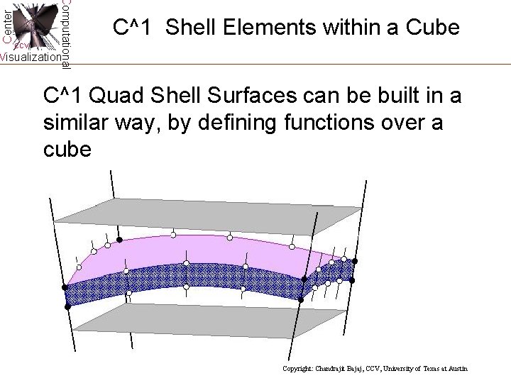
Center Computational CCV C^1 Shell Elements within a Cube Visualization C^1 Quad Shell Surfaces can be built in a similar way, by defining functions over a cube Copyright: Chandrajit Bajaj, CCV, University of Texas at Austin