CENG 538 Advanced Graphics and UIs Curves and

CENG 538 Advanced Graphics and UIs Curves and Surfaces

Various Object Representations • Types of objects: geometrical shapes, trees, terrains, clouds, rocks, glass, hair, furniture, human body, etc. • Not possible to have a single representation for all – Polygon surfaces – Spline surfaces – Procedural methods – Physical models – Solid object models – Fractals – …… 2

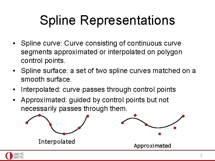
Spline Representations • Spline curve: Curve consisting of continuous curve segments approximated or interpolated on polygon control points. • Spline surface: a set of two spline curves matched on a smooth surface. • Interpolated: curve passes through control points • Approximated: guided by control points but not necessarily passes through them. Interpolated Approximated 3

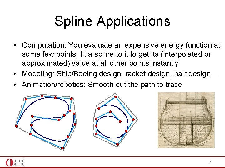
Spline Applications • Computation: You evaluate an expensive energy function at some few points; fit a spline to it to get its (interpolated or approximated) value at all other points instantly • Modeling: Ship/Boeing design, racket design, hair design, . . • Animation/robotics: Smooth out the path to trace 4

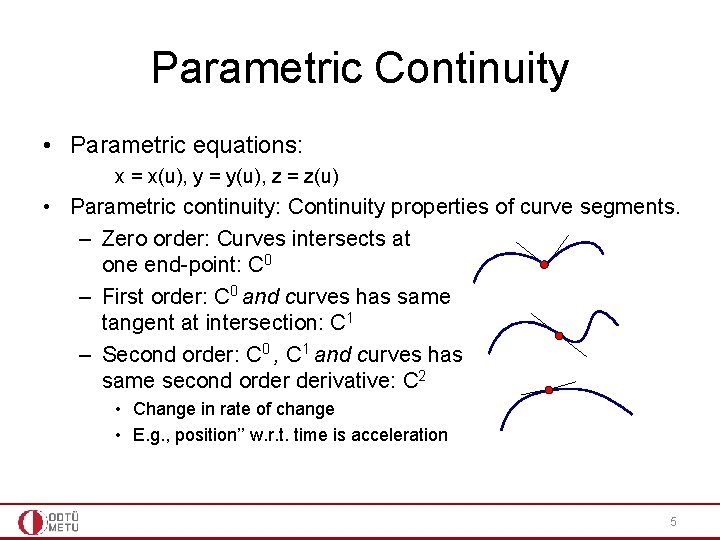
Parametric Continuity • Parametric equations: x = x(u), y = y(u), z = z(u) • Parametric continuity: Continuity properties of curve segments. – Zero order: Curves intersects at one end-point: C 0 – First order: C 0 and curves has same tangent at intersection: C 1 – Second order: C 0 , C 1 and curves has same second order derivative: C 2 • Change in rate of change • E. g. , position’’ w. r. t. time is acceleration 5

Geometric Continuity • Similar to parametric continuity but only the direction of derivatives are significant. For example derivative (1, 2) and (3, 6) are considered equal. • G 0, G 1, G 2 : zero order, first order, and second order geometric continuity. 6

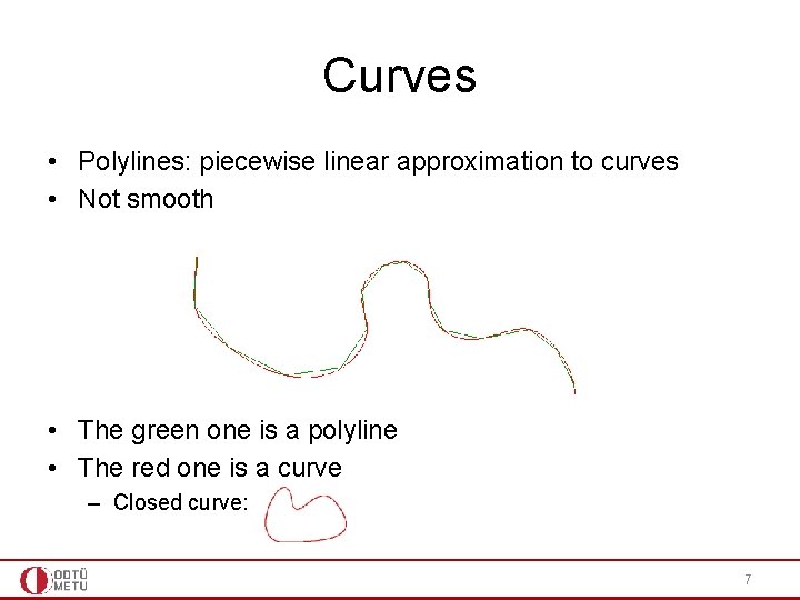
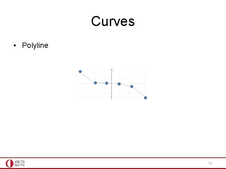
Curves • Polylines: piecewise linear approximation to curves • Not smooth • The green one is a polyline • The red one is a curve – Closed curve: 7

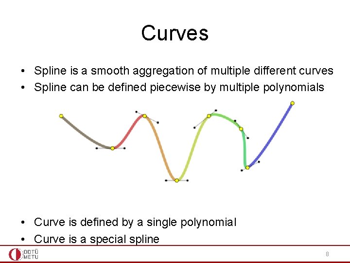
Curves • Spline is a smooth aggregation of multiple different curves • Spline can be defined piecewise by multiple polynomials • Curve is defined by a single polynomial • Curve is a special spline 8

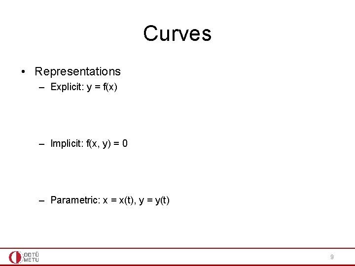
Curves • Representations – Explicit: y = f(x) – Implicit: f(x, y) = 0 – Parametric: x = x(t), y = y(t) 9

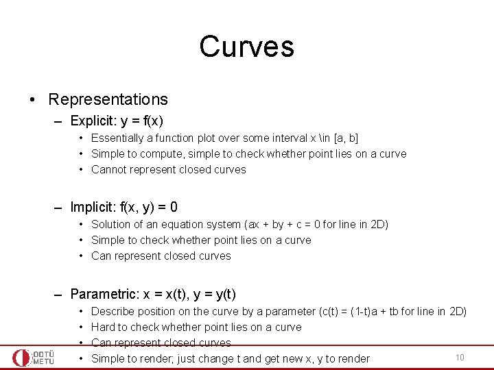
Curves • Representations – Explicit: y = f(x) • Essentially a function plot over some interval x in [a, b] • Simple to compute, simple to check whether point lies on a curve • Cannot represent closed curves – Implicit: f(x, y) = 0 • Solution of an equation system (ax + by + c = 0 for line in 2 D) • Simple to check whether point lies on a curve • Can represent closed curves – Parametric: x = x(t), y = y(t) • • Describe position on the curve by a parameter (c(t) = (1 -t)a + tb for line in 2 D) Hard to check whether point lies on a curve Can represent closed curves 10 Simple to render; just change t and get new x, y to render

Curves • Polyline 11

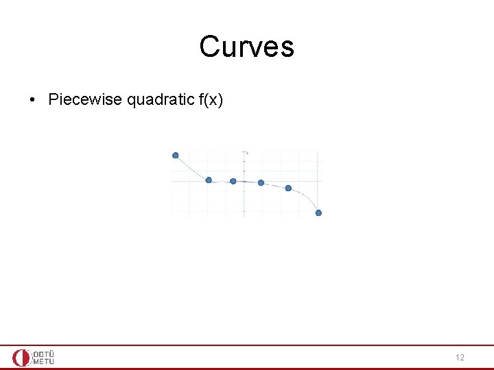
Curves • Piecewise quadratic f(x) 12

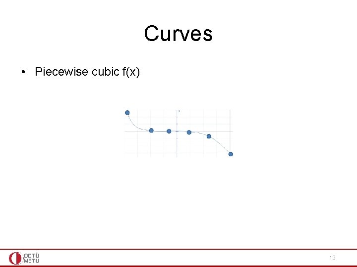
Curves • Piecewise cubic f(x) 13

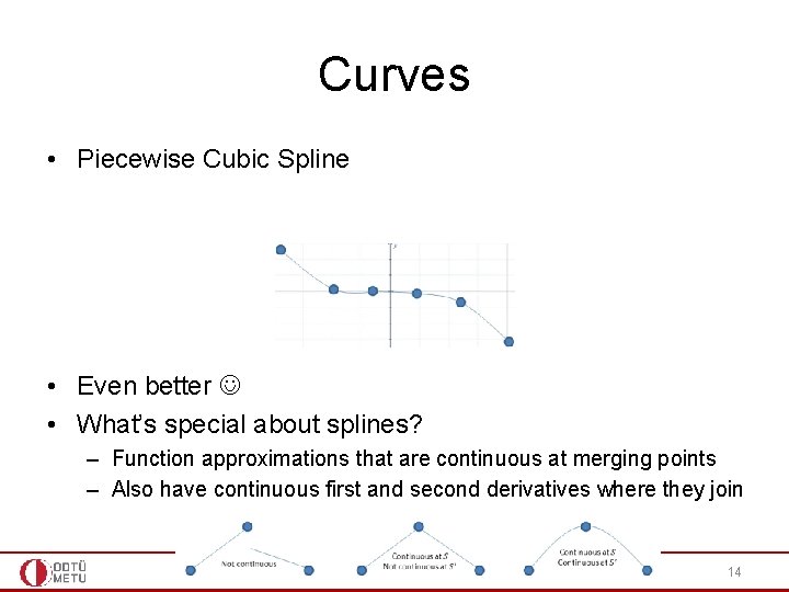
Curves • Piecewise Cubic Spline • Even better • What’s special about splines? – Function approximations that are continuous at merging points – Also have continuous first and second derivatives where they join 14

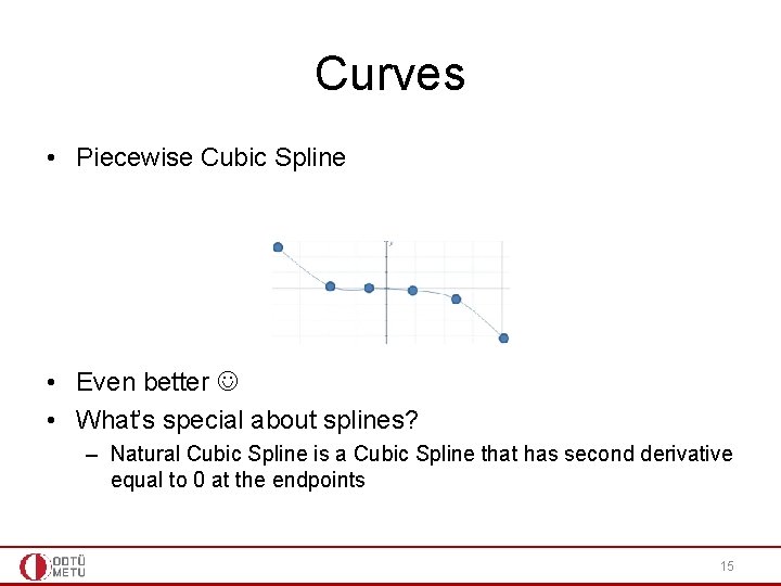
Curves • Piecewise Cubic Spline • Even better • What’s special about splines? – Natural Cubic Spline is a Cubic Spline that has second derivative equal to 0 at the endpoints 15

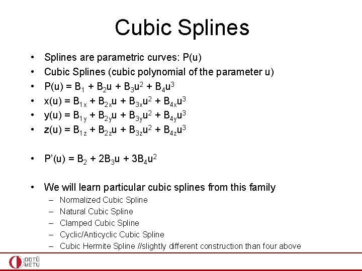
Cubic Splines • • • Splines are parametric curves: P(u) Cubic Splines (cubic polynomial of the parameter u) P(u) = B 1 + B 2 u + B 3 u 2 + B 4 u 3 x(u) = B 1 x + B 2 xu + B 3 xu 2 + B 4 xu 3 y(u) = B 1 y + B 2 yu + B 3 yu 2 + B 4 yu 3 z(u) = B 1 z + B 2 zu + B 3 zu 2 + B 4 zu 3 • P’(u) = B 2 + 2 B 3 u + 3 B 4 u 2 • We will learn particular cubic splines from this family – – – Normalized Cubic Spline Natural Cubic Spline Clamped Cubic Spline Cyclic/Anticyclic Cubic Spline Cubic Hermite Spline //slightly different construction than four above

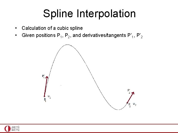
Spline Interpolation • Calculation of a cubic spline • Given positions P 1, P 2, and derivatives/tangents P’ 1, P’ 2

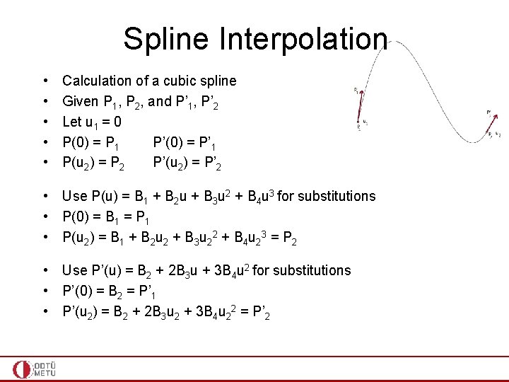
Spline Interpolation • • • Calculation of a cubic spline Given P 1, P 2, and P’ 1, P’ 2 Let u 1 = 0 P(0) = P 1 P’(0) = P’ 1 P(u 2) = P 2 P’(u 2) = P’ 2 • Use P(u) = B 1 + B 2 u + B 3 u 2 + B 4 u 3 for substitutions • P(0) = B 1 = P 1 • P(u 2) = B 1 + B 2 u 2 + B 3 u 22 + B 4 u 23 = P 2 • Use P’(u) = B 2 + 2 B 3 u + 3 B 4 u 2 for substitutions • P’(0) = B 2 = P’ 1 • P’(u 2) = B 2 + 2 B 3 u 2 + 3 B 4 u 22 = P’ 2

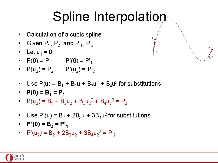
Spline Interpolation • • • Calculation of a cubic spline Given P 1, P 2, and P’ 1, P’ 2 Let u 1 = 0 P(0) = P 1 P’(0) = P’ 1 P(u 2) = P 2 P’(u 2) = P’ 2 • Use P(u) = B 1 + B 2 u + B 3 u 2 + B 4 u 3 for substitutions • P(0) = B 1 = P 1 • P(u 2) = B 1 + B 2 u 2 + B 3 u 22 + B 4 u 23 = P 2 • Use P’(u) = B 2 + 2 B 3 u + 3 B 4 u 2 for substitutions • P’(0) = B 2 = P’ 1 • P’(u 2) = B 2 + 2 B 3 u 2 + 3 B 4 u 22 = P’ 2

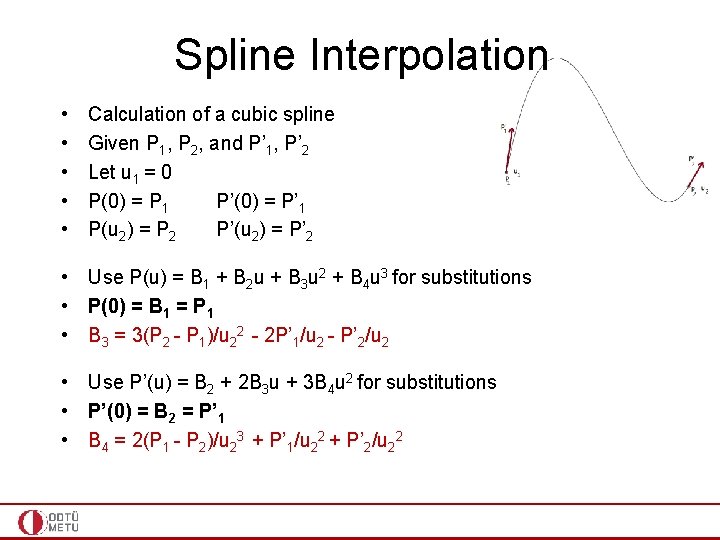
Spline Interpolation • • • Calculation of a cubic spline Given P 1, P 2, and P’ 1, P’ 2 Let u 1 = 0 P(0) = P 1 P’(0) = P’ 1 P(u 2) = P 2 P’(u 2) = P’ 2 • Use P(u) = B 1 + B 2 u + B 3 u 2 + B 4 u 3 for substitutions • P(0) = B 1 = P 1 • B 3 = 3(P 2 - P 1)/u 22 - 2 P’ 1/u 2 - P’ 2/u 2 • Use P’(u) = B 2 + 2 B 3 u + 3 B 4 u 2 for substitutions • P’(0) = B 2 = P’ 1 • B 4 = 2(P 1 - P 2)/u 23 + P’ 1/u 22 + P’ 2/u 22

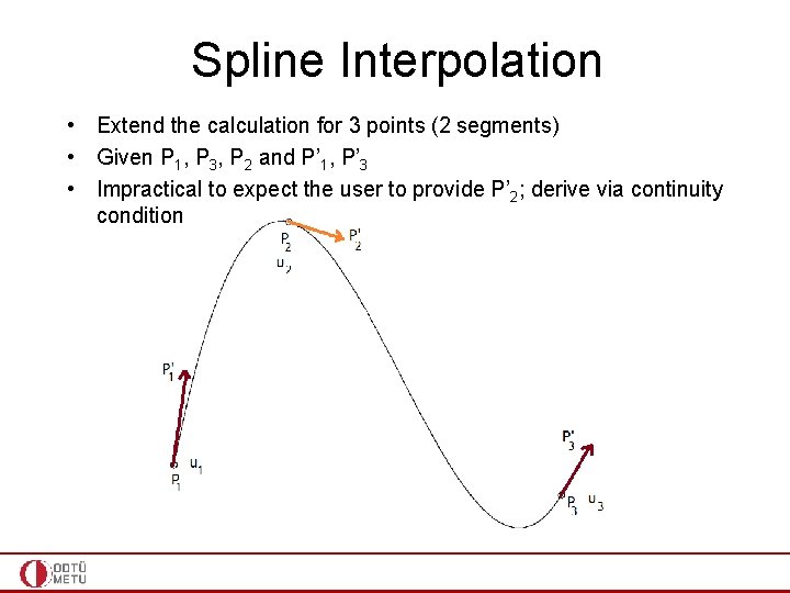
Spline Interpolation • Extend the calculation for 3 points (2 segments) • Given P 1, P 3, P 2 and P’ 1, P’ 3 • Impractical to expect the user to provide P’ 2; derive via continuity condition

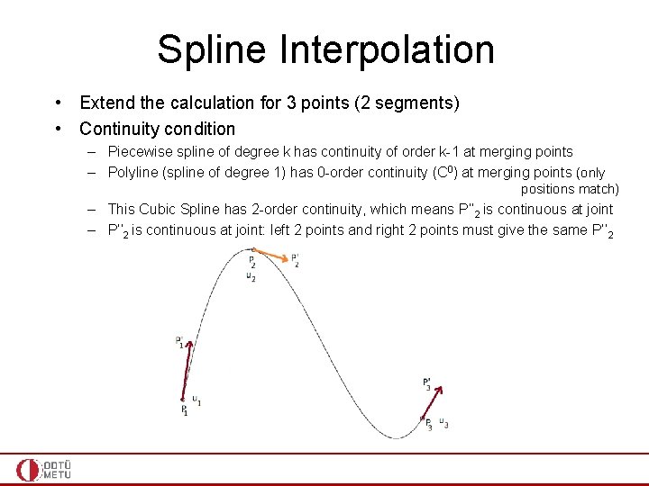
Spline Interpolation • Extend the calculation for 3 points (2 segments) • Continuity condition – Piecewise spline of degree k has continuity of order k-1 at merging points – Polyline (spline of degree 1) has 0 -order continuity (C 0) at merging points (only positions match) – This Cubic Spline has 2 -order continuity, which means P’’ 2 is continuous at joint – P’’ 2 is continuous at joint: left 2 points and right 2 points must give the same P’’ 2

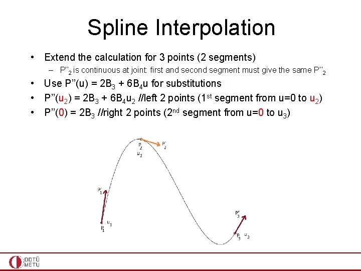
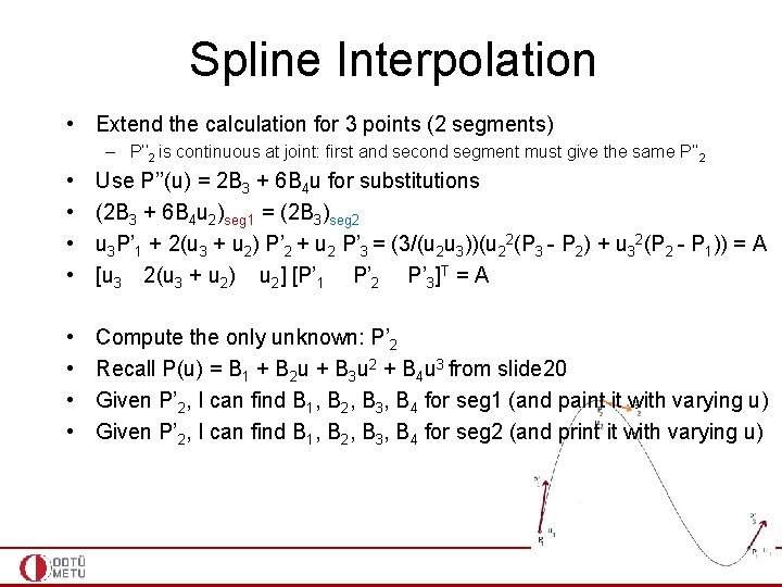
Spline Interpolation • Extend the calculation for 3 points (2 segments) – P’’ 2 is continuous at joint: first and second segment must give the same P’’ 2 • Use P’’(u) = 2 B 3 + 6 B 4 u for substitutions • P’’(u 2) = 2 B 3 + 6 B 4 u 2 //left 2 points (1 st segment from u=0 to u 2) • P’’(0) = 2 B 3 //right 2 points (2 nd segment from u=0 to u 3)

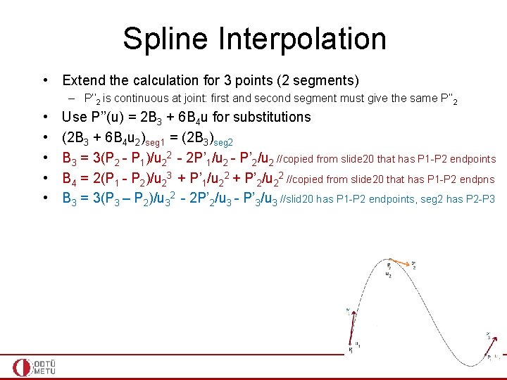
Spline Interpolation • Extend the calculation for 3 points (2 segments) – P’’ 2 is continuous at joint: first and second segment must give the same P’’ 2 • • • Use P’’(u) = 2 B 3 + 6 B 4 u for substitutions (2 B 3 + 6 B 4 u 2)seg 1 = (2 B 3)seg 2 B 3 = 3(P 2 - P 1)/u 22 - 2 P’ 1/u 2 - P’ 2/u 2 //copied from slide 20 that has P 1 -P 2 endpoints B 4 = 2(P 1 - P 2)/u 23 + P’ 1/u 22 + P’ 2/u 22 //copied from slide 20 that has P 1 -P 2 endpns B 3 = 3(P 3 – P 2)/u 32 - 2 P’ 2/u 3 - P’ 3/u 3 //slid 20 has P 1 -P 2 endpoints, seg 2 has P 2 -P 3

Spline Interpolation • Extend the calculation for 3 points (2 segments) – P’’ 2 is continuous at joint: first and second segment must give the same P’’ 2 • • Use P’’(u) = 2 B 3 + 6 B 4 u for substitutions (2 B 3 + 6 B 4 u 2)seg 1 = (2 B 3)seg 2 u 3 P’ 1 + 2(u 3 + u 2) P’ 2 + u 2 P’ 3 = (3/(u 2 u 3))(u 22(P 3 - P 2) + u 32(P 2 - P 1)) = A [u 3 2(u 3 + u 2) u 2] [P’ 1 P’ 2 P’ 3]T = A • • Compute the only unknown: P’ 2 Recall P(u) = B 1 + B 2 u + B 3 u 2 + B 4 u 3 from slide 20 Given P’ 2, I can find B 1, B 2, B 3, B 4 for seg 1 (and paint it with varying u) Given P’ 2, I can find B 1, B 2, B 3, B 4 for seg 2 (and print it with varying u)

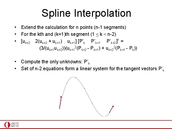
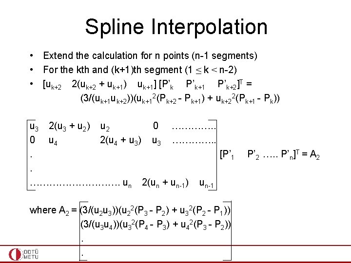
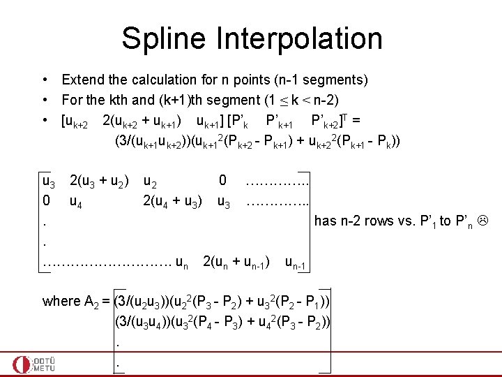
Spline Interpolation • Extend the calculation for n points (n-1 segments) • For the kth and (k+1)th segment (1 ≤ k < n-2) • [uk+2 2(uk+2 + uk+1) uk+1] [P’k P’k+1 P’k+2]T = (3/(uk+1 uk+2))(uk+12(Pk+2 - Pk+1) + uk+22(Pk+1 - Pk)) • Compute the only unknowns: P’k • Set of n-2 equations form a linear system for the tangent vectors P’k

Spline Interpolation • Extend the calculation for n points (n-1 segments) • For the kth and (k+1)th segment (1 ≤ k < n-2) • [uk+2 2(uk+2 + uk+1) uk+1] [P’k P’k+1 P’k+2]T = (3/(uk+1 uk+2))(uk+12(Pk+2 - Pk+1) + uk+22(Pk+1 - Pk)) u 3 2(u 3 + u 2) u 2 0 …………. . 0 u 4 2(u 4 + u 3) u 3 …………. . . [P’ 1. ……………. un 2(un + un-1) un-1 where A 2 = (3/(u 2 u 3))(u 22(P 3 - P 2) + u 32(P 2 - P 1)) (3/(u 3 u 4))(u 32(P 4 - P 3) + u 42(P 3 - P 2)). . P’ 2 …. . P’n]T = A 2

Spline Interpolation • Extend the calculation for n points (n-1 segments) • For the kth and (k+1)th segment (1 ≤ k < n-2) • [uk+2 2(uk+2 + uk+1) uk+1] [P’k P’k+1 P’k+2]T = (3/(uk+1 uk+2))(uk+12(Pk+2 - Pk+1) + uk+22(Pk+1 - Pk)) u 3 2(u 3 + u 2) u 2 0 …………. . 0 u 4 2(u 4 + u 3) u 3 …………. . . has n-2 rows vs. P’ 1 to P’n . ……………. un 2(un + un-1) un-1 where A 2 = (3/(u 2 u 3))(u 22(P 3 - P 2) + u 32(P 2 - P 1)) (3/(u 3 u 4))(u 32(P 4 - P 3) + u 42(P 3 - P 2)). .

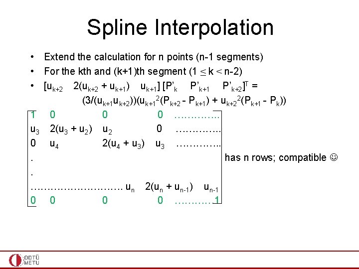
Spline Interpolation • Extend the calculation for n points (n-1 segments) • For the kth and (k+1)th segment (1 ≤ k < n-2) • [uk+2 2(uk+2 + uk+1) uk+1] [P’k P’k+1 P’k+2]T = (3/(uk+1 uk+2))(uk+12(Pk+2 - Pk+1) + uk+22(Pk+1 - Pk)) 1 0 0 0 …………. . u 3 2(u 3 + u 2) u 2 0 …………. . 0 u 4 2(u 4 + u 3) u 3 …………. . . has n rows; compatible . ……………. un 2(un + un-1) un-1 0 0 ………… 1

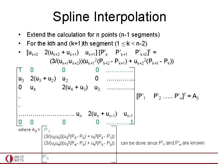
Spline Interpolation • Extend the calculation for n points (n-1 segments) • For the kth and (k+1)th segment (1 ≤ k < n-2) • [uk+2 2(uk+2 + uk+1) uk+1] [P’k P’k+1 P’k+2]T = (3/(uk+1 uk+2))(uk+12(Pk+2 - Pk+1) + uk+22(Pk+1 - Pk)) 1 0 0 0 …………. . u 3 2(u 3 + u 2) u 2 0 …………. . 0 u 4 2(u 4 + u 3) u 3 …………. . . [P’ 1 P’ 2 …. . P’n]T = A 3. ……………. un 2(un + un-1) un-1 0 0 ………… 1 where A 3 = P’ 1 (3/(u 2 u 3))(u 22(P 3 - P 2) + u 32(P 2 - P 1)) (3/(u 3 u 4))(u 32(P 4 - P 3) + u 42(P 3 - P 2)). P’n can be done since P’ 1 and P’n are known

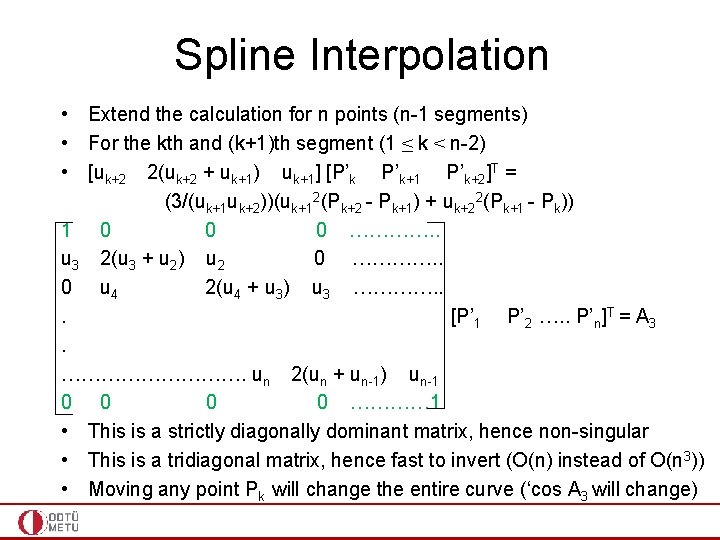
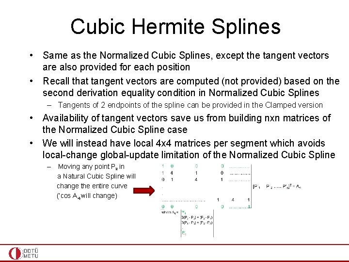
Spline Interpolation • Extend the calculation for n points (n-1 segments) • For the kth and (k+1)th segment (1 ≤ k < n-2) • [uk+2 2(uk+2 + uk+1) uk+1] [P’k P’k+1 P’k+2]T = (3/(uk+1 uk+2))(uk+12(Pk+2 - Pk+1) + uk+22(Pk+1 - Pk)) 1 0 0 0 …………. . u 3 2(u 3 + u 2) u 2 0 …………. . 0 u 4 2(u 4 + u 3) u 3 …………. . . [P’ 1 P’ 2 …. . P’n]T = A 3. ……………. un 2(un + un-1) un-1 0 0 ………… 1 • This is a strictly diagonally dominant matrix, hence non-singular • This is a tridiagonal matrix, hence fast to invert (O(n) instead of O(n 3)) • Moving any point Pk will change the entire curve (‘cos A 3 will change)

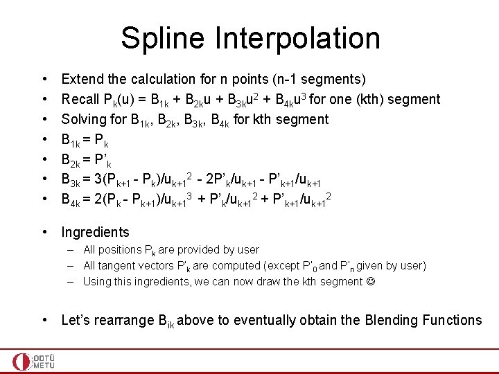
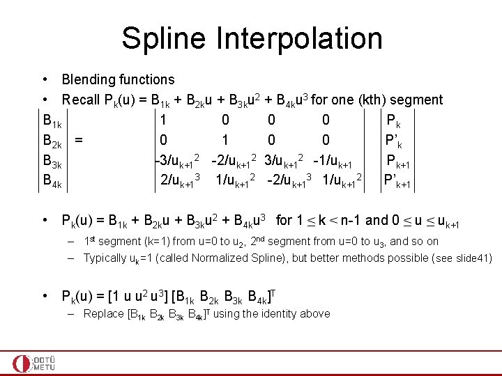
Spline Interpolation • • Extend the calculation for n points (n-1 segments) Recall Pk(u) = B 1 k + B 2 ku + B 3 ku 2 + B 4 ku 3 for one (kth) segment Solving for B 1 k, B 2 k, B 3 k, B 4 k for kth segment B 1 k = Pk B 2 k = P’k B 3 k = 3(Pk+1 - Pk)/uk+12 - 2 P’k/uk+1 - P’k+1/uk+1 B 4 k = 2(Pk - Pk+1)/uk+13 + P’k/uk+12 + P’k+1/uk+12 • Ingredients – All positions Pk are provided by user – All tangent vectors P’k are computed (except P’ 0 and P’n given by user) – Using this ingredients, we can now draw the kth segment • Let’s rearrange Bik above to eventually obtain the Blending Functions

Spline Interpolation • Blending functions • Recall Pk(u) = B 1 k + B 2 ku + B 3 ku 2 + B 4 ku 3 for one (kth) segment B 1 k 1 0 0 0 Pk B 2 k = 0 1 0 0 P’k B 3 k -3/uk+12 -2/uk+12 3/uk+12 -1/uk+1 Pk+1 B 4 k 2/uk+13 1/uk+12 -2/uk+13 1/uk+12 P’k+1 • Pk(u) = B 1 k + B 2 ku + B 3 ku 2 + B 4 ku 3 for 1 ≤ k < n-1 and 0 ≤ uk+1 – 1 st segment (k=1) from u=0 to u 2, 2 nd segment from u=0 to u 3, and so on – Typically uk=1 (called Normalized Spline), but better methods possible (see slide 41) • Pk(u) = [1 u u 2 u 3] [B 1 k B 2 k B 3 k B 4 k]T – Replace [B 1 k B 2 k B 3 k B 4 k]T using the identity above

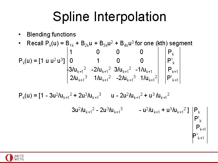
Spline Interpolation • Blending functions • Recall Pk(u) = B 1 k + B 2 ku + B 3 ku 2 + B 4 ku 3 for one (kth) segment 1 0 0 0 Pk Pk(u) = [1 u u 2 u 3] 0 1 0 0 P’k -3/uk+12 -2/uk+12 3/uk+12 -1/uk+1 Pk+1 2/uk+13 1/uk+12 -2/uk+13 1/uk+12 P’k+1 Pk(u) = [1 - 3 u 2/uk+12 + 2 u 3/uk+13 u - 2 u 2/uk+12 + u 3 /uk+12 3 u 2/uk+12 - 2 u 3/uk+13 - u 2/uk+1 + u 3/uk+12 ] Pk P’k Pk+1 P’k+1

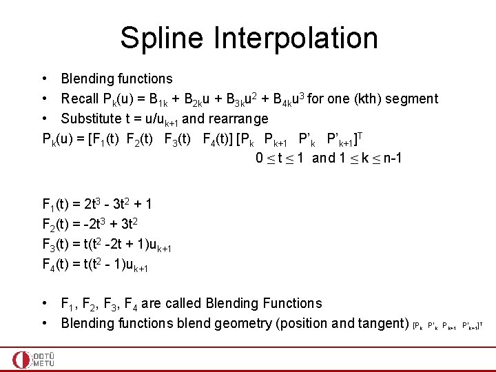
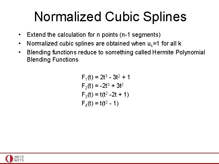
Spline Interpolation • Blending functions • Recall Pk(u) = B 1 k + B 2 ku + B 3 ku 2 + B 4 ku 3 for one (kth) segment • Substitute t = u/uk+1 and rearrange Pk(u) = [F 1(t) F 2(t) F 3(t) F 4(t)] [Pk Pk+1 P’k+1]T 0 ≤ t ≤ 1 and 1 ≤ k ≤ n-1 F 1(t) = 2 t 3 - 3 t 2 + 1 F 2(t) = -2 t 3 + 3 t 2 F 3(t) = t(t 2 -2 t + 1)uk+1 F 4(t) = t(t 2 - 1)uk+1 • F 1, F 2, F 3, F 4 are called Blending Functions • Blending functions blend geometry (position and tangent) [P k P’k Pk+1 P’k+1]T

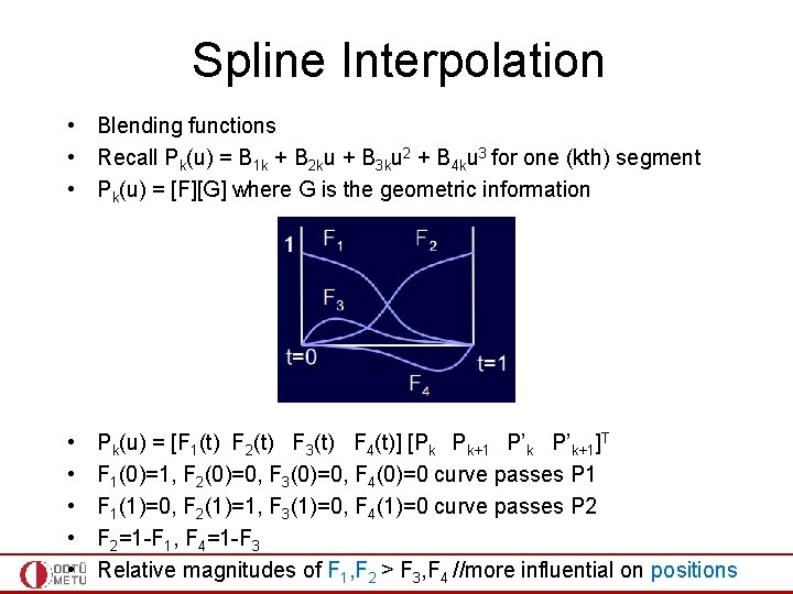
Spline Interpolation • Blending functions • Recall Pk(u) = B 1 k + B 2 ku + B 3 ku 2 + B 4 ku 3 for one (kth) segment • Pk(u) = [F][G] where G is the geometric information • • • Pk(u) = [F 1(t) F 2(t) F 3(t) F 4(t)] [Pk Pk+1 P’k+1]T F 1(0)=1, F 2(0)=0, F 3(0)=0, F 4(0)=0 curve passes P 1 F 1(1)=0, F 2(1)=1, F 3(1)=0, F 4(1)=0 curve passes P 2 F 2=1 -F 1, F 4=1 -F 3 Relative magnitudes of F 1, F 2 > F 3, F 4 //more influential on positions

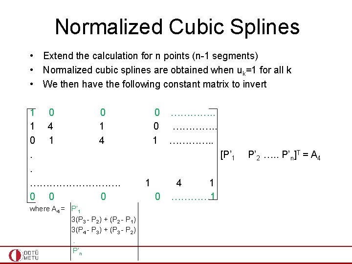
Normalized Cubic Splines • Extend the calculation for n points (n-1 segments) • Normalized cubic splines are obtained when uk=1 for all k • We then have the following constant matrix to invert 1 0 0 1 4 1 0 1 4. . ……………. 0 0 0 where A 4 = P’ 1 3(P 3 - P 2) + (P 2 - P 1) 3(P 4 - P 3) + (P 3 - P 2). P’n 0 …………. . 1 …………. . [P’ 1 1 0 4 1 ………… 1 P’ 2 …. . P’n]T = A 4

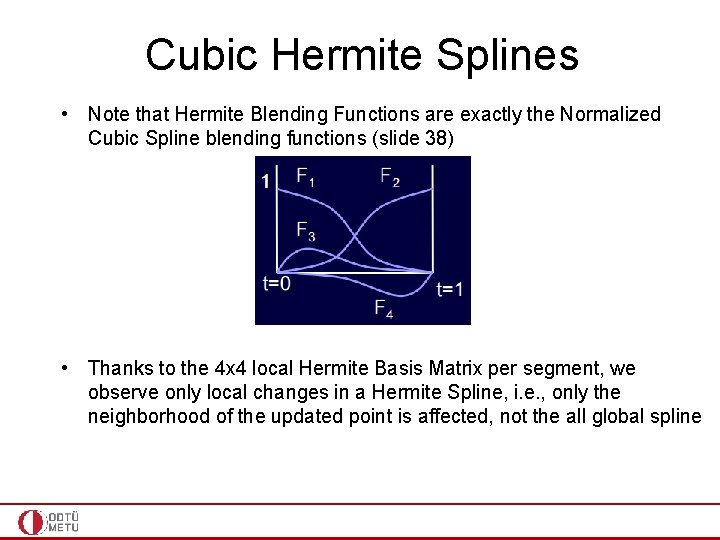
Normalized Cubic Splines • Extend the calculation for n points (n-1 segments) • Normalized cubic splines are obtained when uk=1 for all k • Blending functions reduce to something called Hermite Polynomial Blending Functions F 1(t) = 2 t 3 - 3 t 2 + 1 F 2(t) = -2 t 3 + 3 t 2 F 3(t) = t(t 2 -2 t + 1) F 4(t) = t(t 2 - 1)

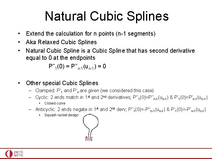
Natural Cubic Splines • Extend the calculation for n points (n-1 segments) • Aka Relaxed Cubic Splines • Natural Cubic Spline is a Cubic Spline that has second derivative equal to 0 at the endpoints P’’ 1(0) = P’’n-1(un-1) = 0 • Other special Cubic Splines – Clamped: P’ 1 and P’n are given (we considered this case) – Cyclic: 2 ends match in 1 st and 2 nd derivatives; P’’ 1(0)=P’’n-1(un-1) & P’ 1(0)=P’n-1(un-1) • Closed curve – Anticyclic: 2 ends negate in 1 st and 2 nd derv; P’’ 1(0)=-P’’n-1(un-1) & P’ 1(0)=-P’n-1(un-1) • Squash racket design

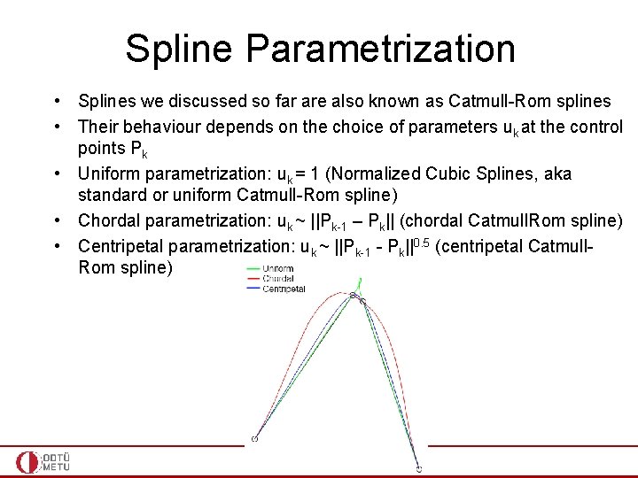
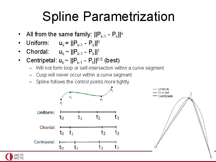
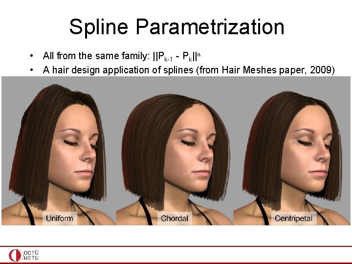
Spline Parametrization • Splines we discussed so far are also known as Catmull-Rom splines • Their behaviour depends on the choice of parameters uk at the control points Pk • Uniform parametrization: uk = 1 (Normalized Cubic Splines, aka standard or uniform Catmull-Rom spline) • Chordal parametrization: uk ~ ||Pk-1 – Pk|| (chordal Catmull. Rom spline) • Centripetal parametrization: uk ~ ||Pk-1 - Pk||0. 5 (centripetal Catmull. Rom spline)

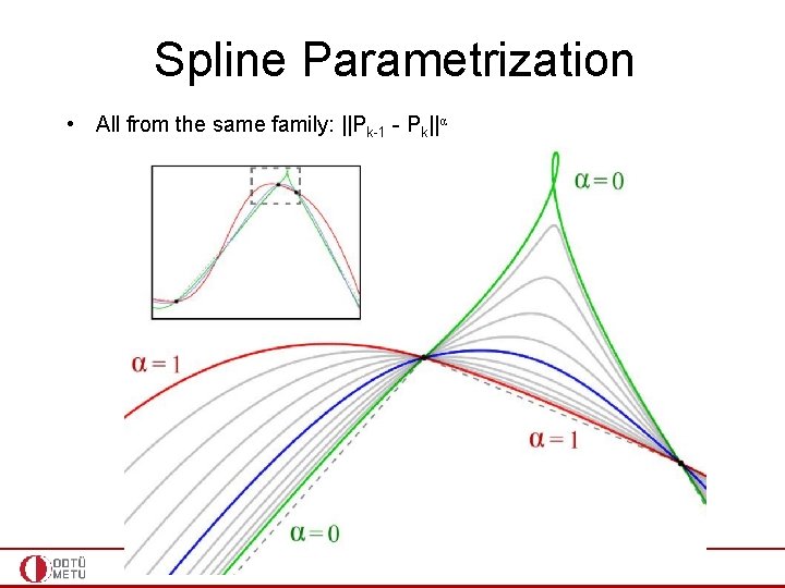
Spline Parametrization • • All from the same family: ||Pk-1 - Pk||α Uniform: uk = ||Pk-1 - Pk||0 Chordal: uk ~ ||Pk-1 - Pk||1 Centripetal: uk ~ ||Pk-1 - Pk||0. 5 (best) – Will not form loop or self-intersection within a curve segment – Cusp will never occur within a curve segment – Spline follows the control points more tightly

Spline Parametrization • All from the same family: ||Pk-1 - Pk||α

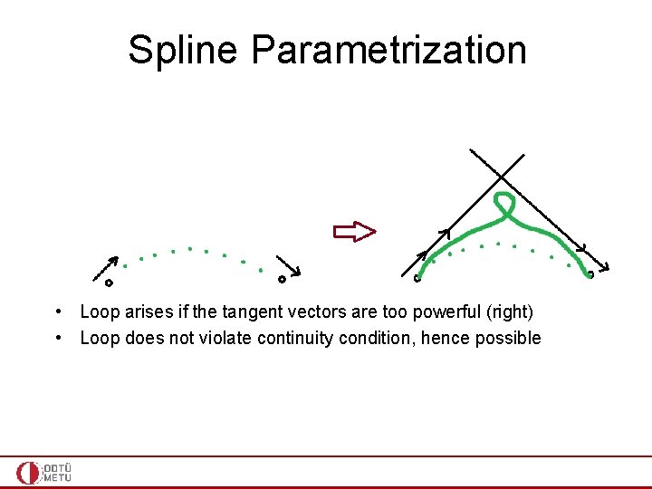
Spline Parametrization • Loop arises if the tangent vectors are too powerful (right) • Loop does not violate continuity condition, hence possible

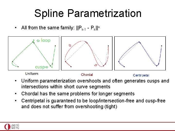
Spline Parametrization • All from the same family: ||Pk-1 - Pk||α • Uniform parameterization overshoots and often generates cusps and intersections within short curve segments • Chordal has the same problems for longer segments • Centripetal is guaranteed to be loop/intersection-free and cusp-free and does not suffer from overshooting (tight)

Spline Parametrization • All from the same family: ||Pk-1 - Pk||α • A hair design application of splines (from Hair Meshes paper, 2009)

Cubic Hermite Splines • Same as the Normalized Cubic Splines, except the tangent vectors are also provided for each position • Recall that tangent vectors are computed (not provided) based on the second derivation equality condition in Normalized Cubic Splines – Tangents of 2 endpoints of the spline can be provided in the Clamped version • Availability of tangent vectors save us from building nxn matrices of the Normalized Cubic Spline case • We will instead have local 4 x 4 matrices per segment which avoids local-change global-update limitation of the Normalized Cubic Spline – Moving any point Pk in a Natural Cubic Spline will change the entire curve (‘cos A 4 will change)

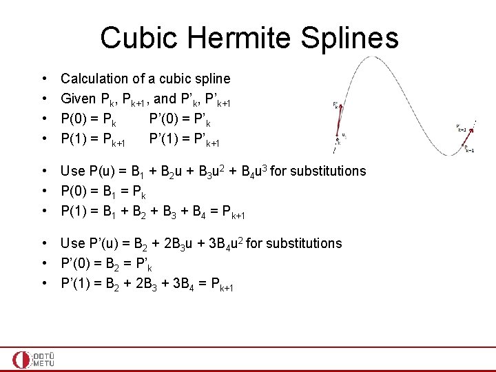
Cubic Hermite Splines • • Calculation of a cubic spline Given Pk, Pk+1, and P’k, P’k+1 P(0) = Pk P’(0) = P’k P(1) = Pk+1 P’(1) = P’k+1 • Use P(u) = B 1 + B 2 u + B 3 u 2 + B 4 u 3 for substitutions • P(0) = B 1 = Pk • P(1) = B 1 + B 2 + B 3 + B 4 = Pk+1 • Use P’(u) = B 2 + 2 B 3 u + 3 B 4 u 2 for substitutions • P’(0) = B 2 = P’k • P’(1) = B 2 + 2 B 3 + 3 B 4 = Pk+1

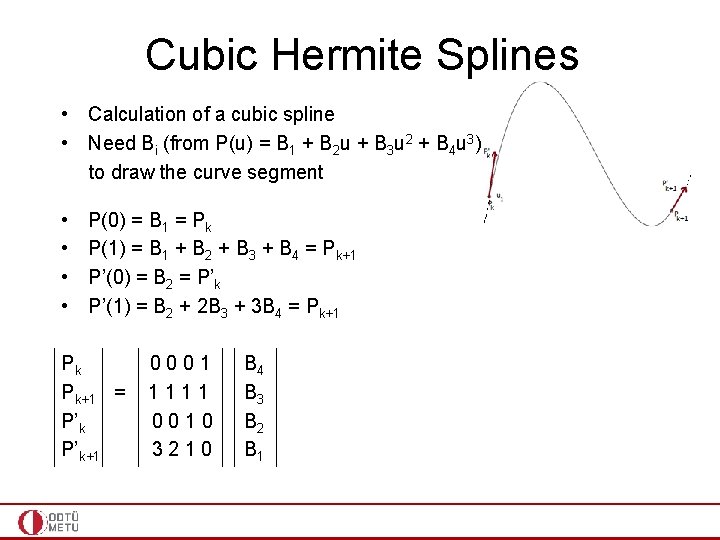
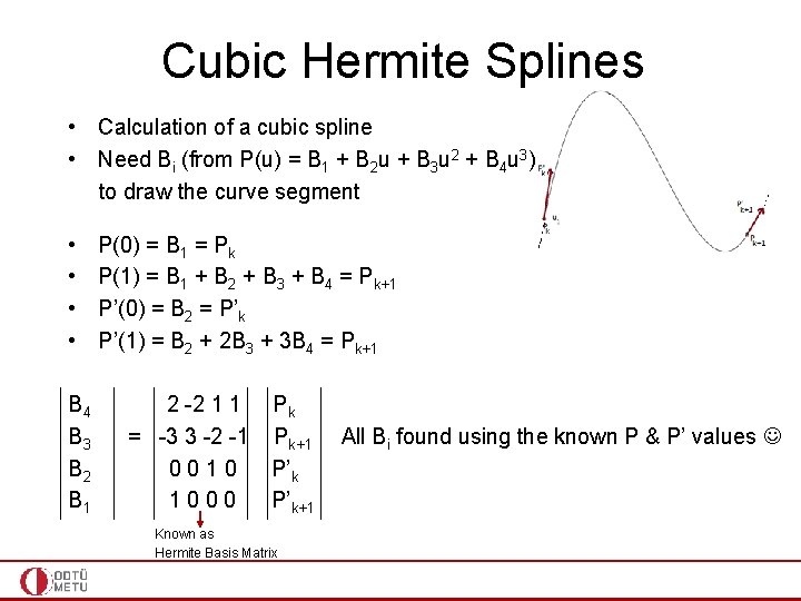
Cubic Hermite Splines • Calculation of a cubic spline • Need Bi (from P(u) = B 1 + B 2 u + B 3 u 2 + B 4 u 3) to draw the curve segment • • P(0) = B 1 = Pk P(1) = B 1 + B 2 + B 3 + B 4 = Pk+1 P’(0) = B 2 = P’k P’(1) = B 2 + 2 B 3 + 3 B 4 = Pk+1 Pk Pk+1 = P’k+1 0001 1111 0010 3210 B 4 B 3 B 2 B 1

Cubic Hermite Splines • Calculation of a cubic spline • Need Bi (from P(u) = B 1 + B 2 u + B 3 u 2 + B 4 u 3) to draw the curve segment • • P(0) = B 1 = Pk P(1) = B 1 + B 2 + B 3 + B 4 = Pk+1 P’(0) = B 2 = P’k P’(1) = B 2 + 2 B 3 + 3 B 4 = Pk+1 -1 B 4 B 3 B 2 B 1 = 0001 1111 0010 3210 Pk Pk+1 P’k+1

Cubic Hermite Splines • Calculation of a cubic spline • Need Bi (from P(u) = B 1 + B 2 u + B 3 u 2 + B 4 u 3) to draw the curve segment • • B 4 B 3 B 2 B 1 P(0) = B 1 = Pk P(1) = B 1 + B 2 + B 3 + B 4 = Pk+1 P’(0) = B 2 = P’k P’(1) = B 2 + 2 B 3 + 3 B 4 = Pk+1 2 -2 1 1 = -3 3 -2 -1 0010 1000 Pk Pk+1 P’k+1 Known as Hermite Basis Matrix All Bi found using the known P & P’ values

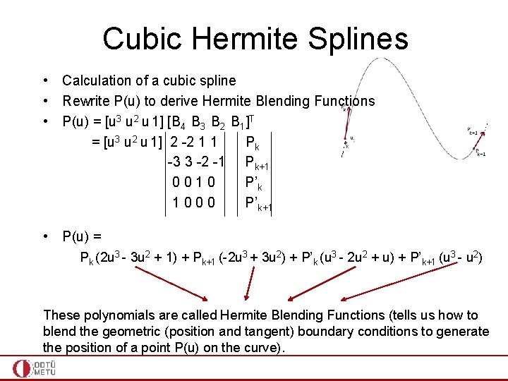
Cubic Hermite Splines • Calculation of a cubic spline • Rewrite P(u) to derive Hermite Blending Functions • P(u) = [u 3 u 2 u 1] [B 4 B 3 B 2 B 1]T = [u 3 u 2 u 1] 2 -2 1 1 Pk -3 3 -2 -1 Pk+1 0010 P’k 1000 P’k+1 • P(u) = Pk (2 u 3 - 3 u 2 + 1) + Pk+1 (-2 u 3 + 3 u 2) + P’k (u 3 - 2 u 2 + u) + P’k+1 (u 3 - u 2) These polynomials are called Hermite Blending Functions (tells us how to blend the geometric (position and tangent) boundary conditions to generate the position of a point P(u) on the curve).

Cubic Hermite Splines • Note that Hermite Blending Functions are exactly the Normalized Cubic Spline blending functions (slide 38) • Thanks to the 4 x 4 local Hermite Basis Matrix per segment, we observe only local changes in a Hermite Spline, i. e. , only the neighborhood of the updated point is affected, not the all global spline

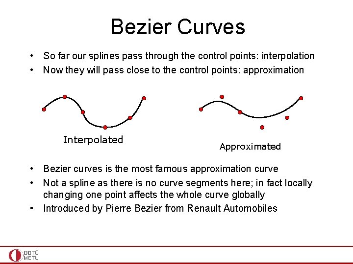
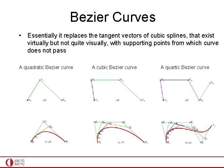
Bezier Curves • So far our splines pass through the control points: interpolation • Now they will pass close to the control points: approximation Interpolated Approximated • Bezier curves is the most famous approximation curve • Not a spline as there is no curve segments here; in fact locally changing one point affects the whole curve globally • Introduced by Pierre Bezier from Renault Automobiles

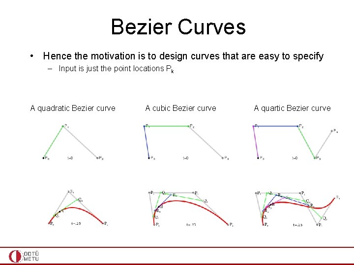
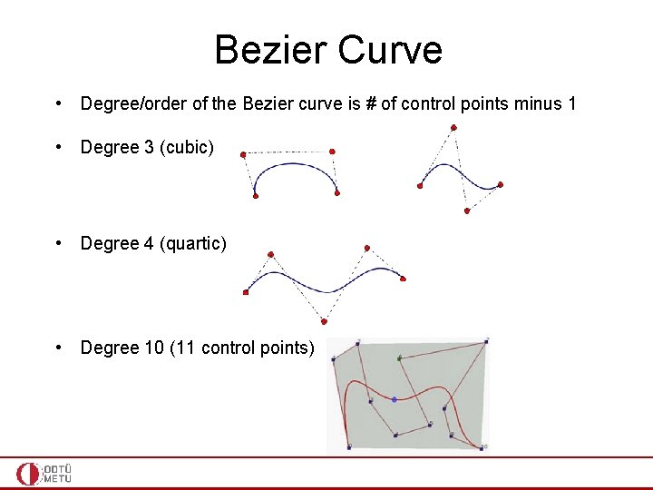
Bezier Curves • Essentially it replaces the tangent vectors of cubic splines, that exist virtually but not quite visually, with supporting points from which curve does not pass A quadratic Bezier curve A cubic Bezier curve A quartic Bezier curve

Bezier Curves • Hence the motivation is to design curves that are easy to specify – Input is just the point locations Pk A quadratic Bezier curve A cubic Bezier curve A quartic Bezier curve

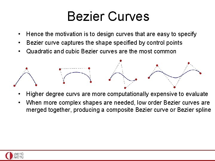
Bezier Curves • Hence the motivation is to design curves that are easy to specify • Bezier curve captures the shape specified by control points • Quadratic and cubic Bezier curves are the most common • Higher degree curvs are more computationally expensive to evaluate • When more complex shapes are needed, low order Bezier curves are merged together, producing a composite Bezier curve or Bezier spline

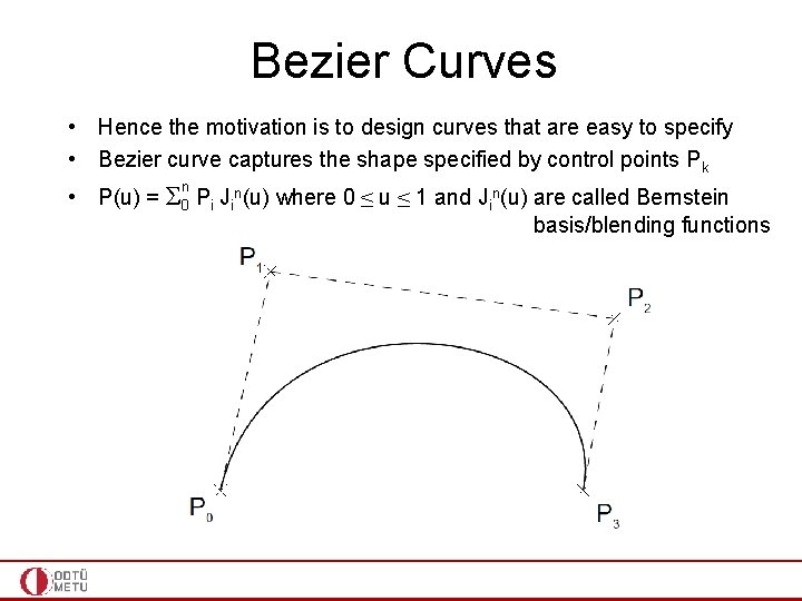
Bezier Curves • Hence the motivation is to design curves that are easy to specify • Bezier curve captures the shape specified by control points Pk n • P(u) = Σ 0 Pi Jin(u) where 0 ≤ u ≤ 1 and Jin(u) are called Bernstein basis/blending functions

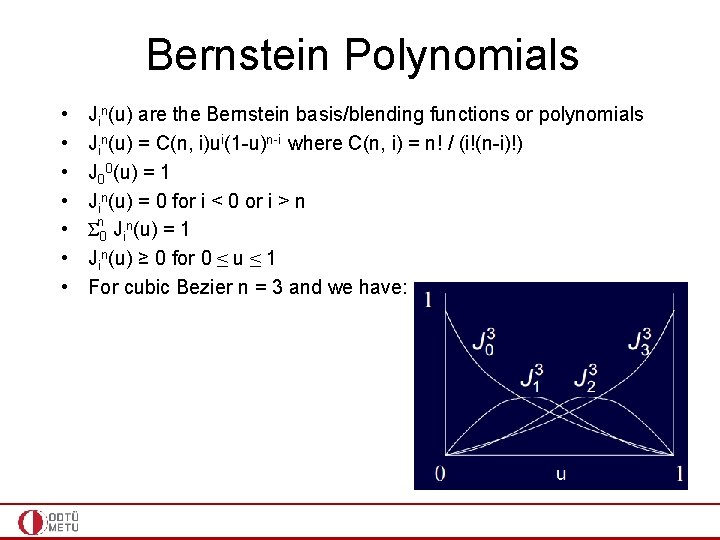
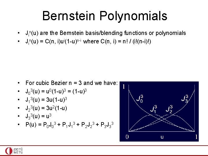
Bernstein Polynomials • • Jin(u) are the Bernstein basis/blending functions or polynomials Jin(u) = C(n, i)ui(1 -u)n-i where C(n, i) = n! / (i!(n-i)!) J 00(u) = 1 Jin(u) = 0 for i < 0 or i > n Σn 0 Jin(u) = 1 Jin(u) ≥ 0 for 0 ≤ u ≤ 1 For cubic Bezier n = 3 and we have:

Bernstein Polynomials • Jin(u) are the Bernstein basis/blending functions or polynomials • Jin(u) = C(n, i)ui(1 -u)n-i where C(n, i) = n! / (i!(n-i)!) • • • For cubic Bezier n = 3 and we have: J 03(u) = u 0(1 -u)3 = (1 -u)3 J 13(u) = 3 u(1 -u)3 J 23(u) = 3 u 2(1 -u) J 33(u) = u 3 P(u) = P 0 J 03 + P 1 J 13 + P 2 J 23 + P 3 J 33

Bezier Curve • Degree/order of the Bezier curve is # of control points minus 1 • Degree 3 (cubic) • Degree 4 (quartic) • Degree 10 (11 control points)

Bezier Curve • End point interpolation property – Bezier curve (of any degree) interpolates the 2 endpoints (passes through) – Recall Jin(u) = C(n, i)ui(1 -u)n-i – – At u=0 (first endpoint) i = 0, J 0 n(0) = C(n, 0)u 0(1 -u)n-0 = 1 i ≠ 0, Jin(0) = C(n, i)0 i(1 -0)n-i = 0 P(0) = P 0 J 0 n(0) = P 0

Bezier Curve • End point interpolation property – Bezier curve (of any degree) interpolates the 2 endpoints (passes through) – Recall Jin(u) = C(n, i)ui(1 -u)n-i – – At u=1 (second endpoint) i = n, Jnn(1) = C(n, n)1 n(1 -u)0 = 1 i ≠ n, Jin(1) = C(n, i)1 i(1 -1)n-i = 0 P(1) = Pn. Jnn(1) = Pn

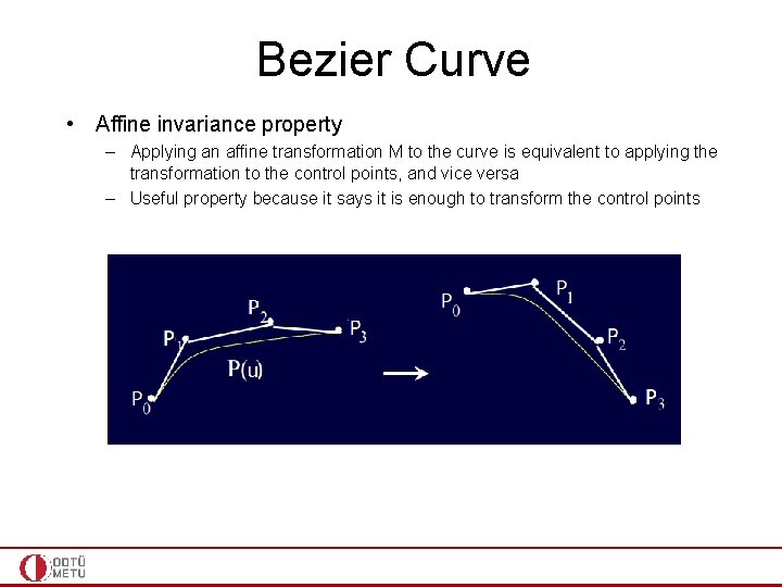
Bezier Curve • Affine invariance property – Applying an affine transformation M to the curve is equivalent to applying the transformation to the control points, and vice versa – Useful property because it says it is enough to transform the control points

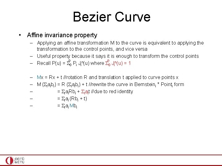
Bezier Curve • Affine invariance property – Applying an affine transformation M to the curve is equivalent to applying the transformation to the control points, and vice versa – Useful property because it says it is enough to transform the control points n n – Recall P(u) = Σ 0 Pi Jin(u) where Σ 0 Jin(u) = 1 – Mx = Rx + t //rotation R and translation t applied to curve points x – M (Σiaibi) = R (Σiaibi) + t //rewrite the curve in Bernsteini * Pointi form – = Σiai. Rbi + Σiait //due to red identity – = Σiai (Rbi + t) – = Σiai Mbi

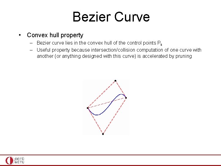
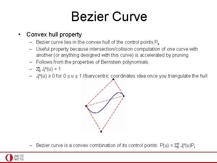
Bezier Curve • Convex hull property – Bezier curve lies in the convex hull of the control points Pk – Useful property because intersection/collision computation of one curve with another (or anything designed with this curve) is accelerated by pruning

Bezier Curve • Convex hull property – Bezier curve lies in the convex hull of the control points Pk – Useful property because intersection/collision computation of one curve with another (or anything designed with this curve) is accelerated by pruning – Follows from the properties of Bernstein polynomials: – Σn 0 Jin(u) = 1 – Jin(u) ≥ 0 for 0 ≤ u ≤ 1 //barycentric coordinates idea once you triangulate the hull – Bezier curve is a convex combination of its control points: P(u) = Σ 0 n Jin(u)Pi

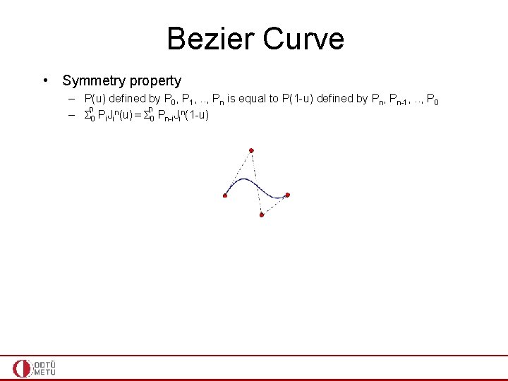
Bezier Curve • Symmetry property – P(u) defined by P 0, P 1, . . , Pn is equal to P(1 -u) defined by Pn, Pn-1, . . , P 0 n n – Σ 0 Pi. Jin(u) = Σ 0 Pn-i. Jin(1 -u)

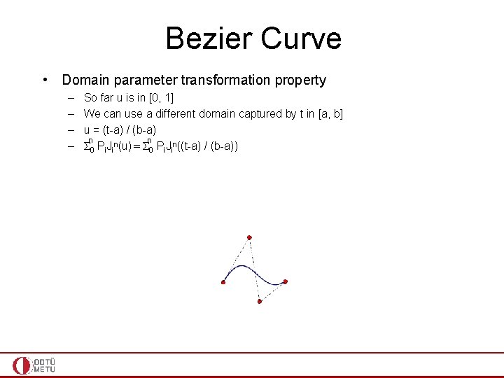
Bezier Curve • Domain parameter transformation property – – So far u is in [0, 1] We can use a different domain captured by t in [a, b] u = (t-a) / (b-a) n n Σ 0 Pi. Jin(u) = Σ 0 Pi. Jin((t-a) / (b-a))

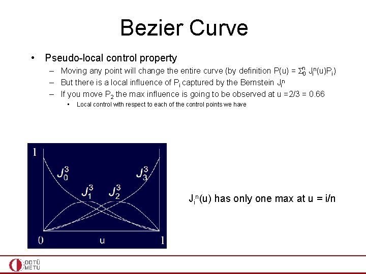
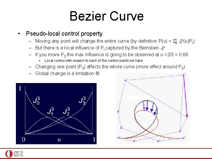
Bezier Curve • Pseudo-local control property – Moving any point will change the entire curve (by definition P(u) = Σn 0 Jin(u)Pi) – But there is a local influence of Pi captured by the Bernstein Jin – If you move P 2 the max influence is going to be observed at u =2/3 = 0. 66 • Local control with respect to each of the control points we have Jin(u) has only one max at u = i/n

Bezier Curve • Pseudo-local control property – Moving any point will change the entire curve (by definition P(u) = Σn 0 Jin(u)Pi) – But there is a local influence of Pi captured by the Bernstein Jin – If you move P 2 the max influence is going to be observed at u =2/3 = 0. 66 • Local control with respect to each of the control points we have – Changing one point (P 3) affects the whole curve (more effect around P 3) – Global change is a limitation

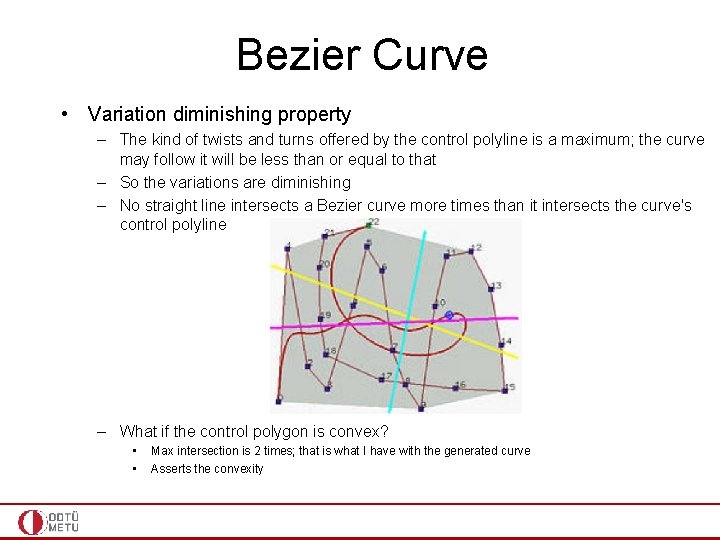
Bezier Curve • Variation diminishing property – The kind of twists and turns offered by the control polyline is a maximum; the curve may follow it will be less than or equal to that – So the variations are diminishing – No straight line intersects a Bezier curve more times than it intersects the curve's control polyline – What if the control polygon is convex? • • Max intersection is 2 times; that is what I have with the generated curve Asserts the convexity

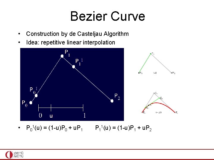
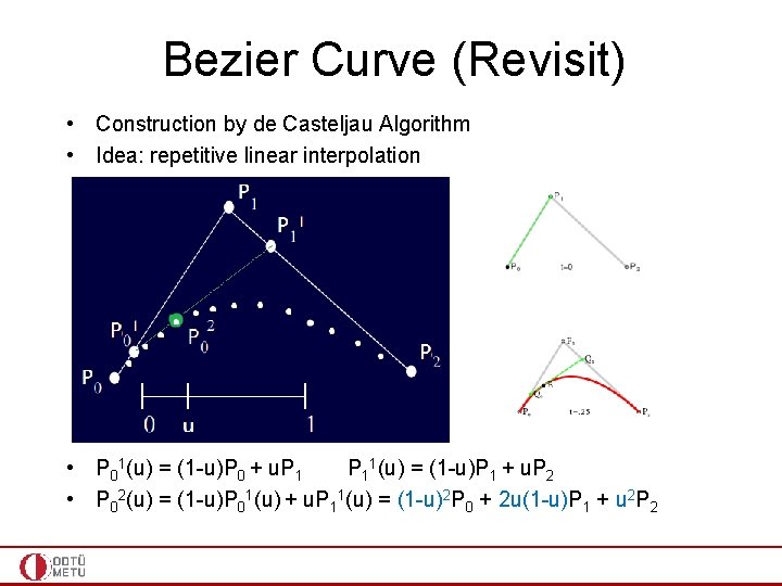
Bezier Curve • Construction by de Casteljau Algorithm • Idea: repetitive linear interpolation • P 01(u) = (1 -u)P 0 + u. P 11(u) = (1 -u)P 1 + u. P 2

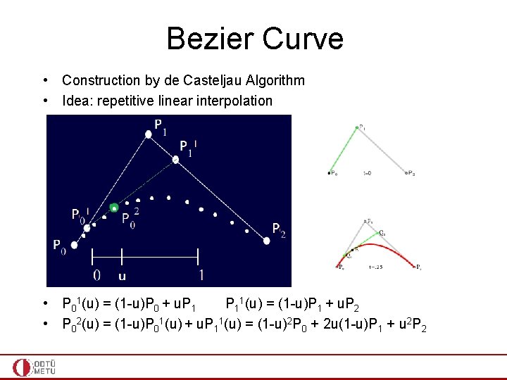
Bezier Curve • Construction by de Casteljau Algorithm • Idea: repetitive linear interpolation • P 01(u) = (1 -u)P 0 + u. P 11(u) = (1 -u)P 1 + u. P 2 • P 02(u) = (1 -u)P 01(u) + u. P 11(u) = (1 -u)2 P 0 + 2 u(1 -u)P 1 + u 2 P 2

Bezier Curve • Construction by de Casteljau Algorithm • Idea: repetitive linear interpolation • P 01(u) = (1 -u)P 0 + u. P 11(u) = (1 -u)P 1 + u. P 2 • P 02(u) = (1 -u)P 01(u) + u. P 11(u) = (1 -u)2 P 0 + 2 u(1 -u)P 1 + u 2 P 2 • Bernstein polynomials of degree 2; so what I get is a Bezier curve

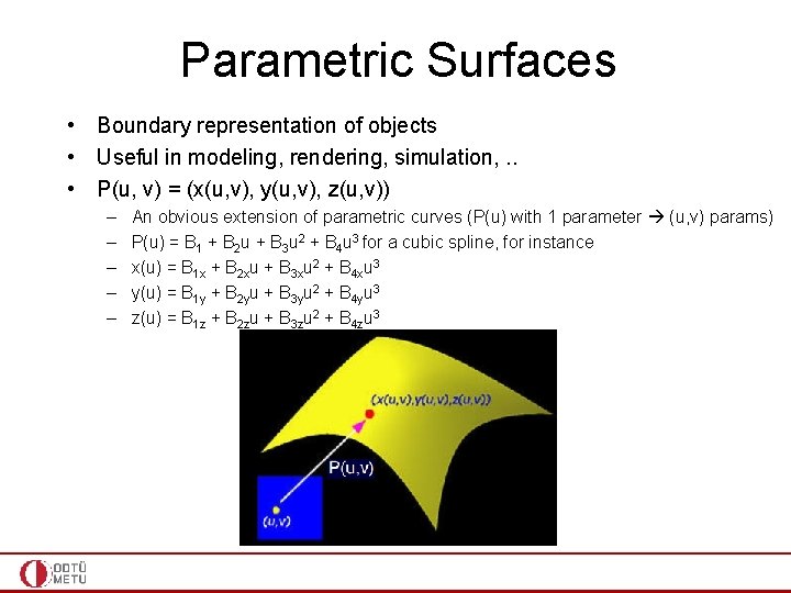
Parametric Surfaces • Boundary representation of objects • Useful in modeling, rendering, simulation, . . • P(u, v) = (x(u, v), y(u, v), z(u, v)) – – – An obvious extension of parametric curves (P(u) with 1 parameter (u, v) params) P(u) = B 1 + B 2 u + B 3 u 2 + B 4 u 3 for a cubic spline, for instance x(u) = B 1 x + B 2 xu + B 3 xu 2 + B 4 xu 3 y(u) = B 1 y + B 2 yu + B 3 yu 2 + B 4 yu 3 z(u) = B 1 z + B 2 zu + B 3 zu 2 + B 4 zu 3

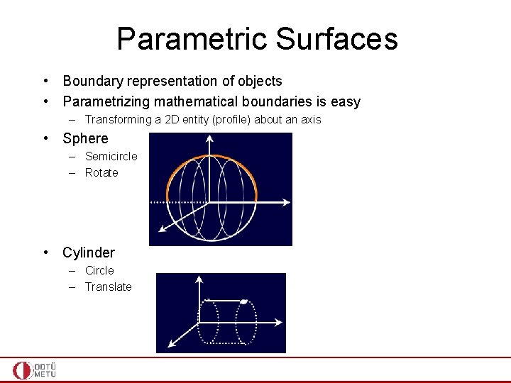
Parametric Surfaces • Boundary representation of objects • Parametrizing mathematical boundaries is easy – Transforming a 2 D entity (profile) about an axis • Sphere – Semicircle – Rotate • Cylinder – Circle – Translate

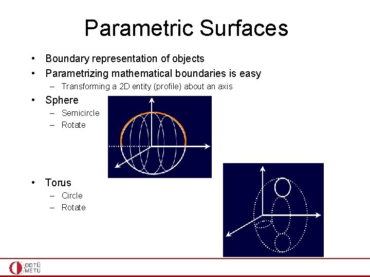
Parametric Surfaces • Boundary representation of objects • Parametrizing mathematical boundaries is easy – Transforming a 2 D entity (profile) about an axis • Sphere – Semicircle – Rotate • Torus – Circle – Rotate

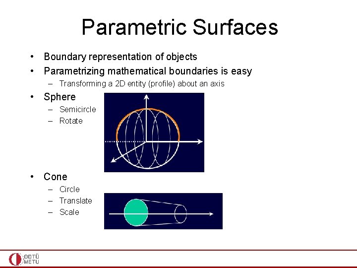
Parametric Surfaces • Boundary representation of objects • Parametrizing mathematical boundaries is easy – Transforming a 2 D entity (profile) about an axis • Sphere – Semicircle – Rotate • Cone – Circle – Translate – Scale

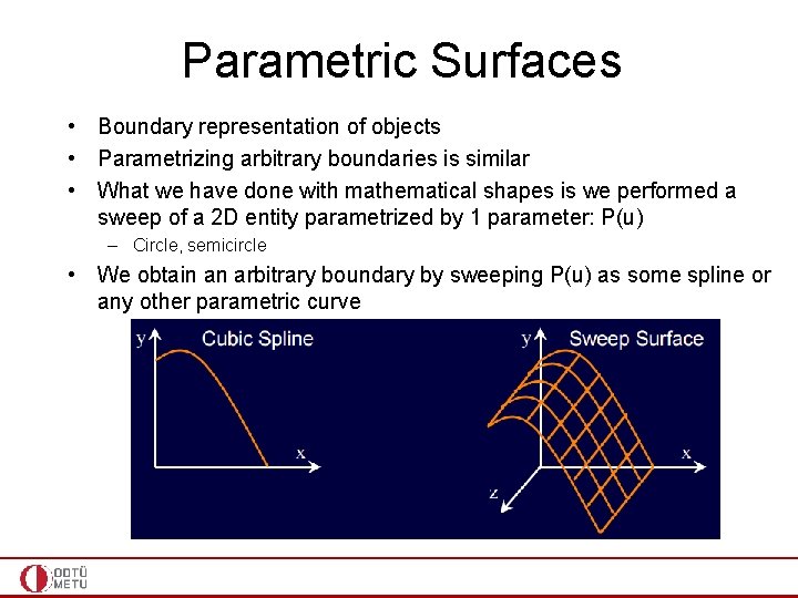
Parametric Surfaces • Boundary representation of objects • Parametrizing arbitrary boundaries is similar • What we have done with mathematical shapes is we performed a sweep of a 2 D entity parametrized by 1 parameter: P(u) – Circle, semicircle • We obtain an arbitrary boundary by sweeping P(u) as some spline or any other parametric curve

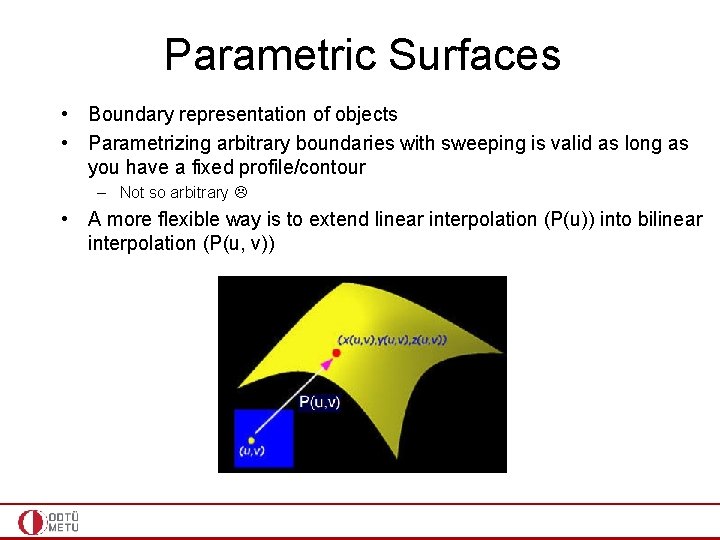
Parametric Surfaces • Boundary representation of objects • Parametrizing arbitrary boundaries with sweeping is valid as long as you have a fixed profile/contour – Not so arbitrary • A more flexible way is to extend linear interpolation (P(u)) into bilinear interpolation (P(u, v))

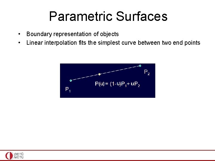
Parametric Surfaces • Boundary representation of objects • Linear interpolation fits the simplest curve between two end points

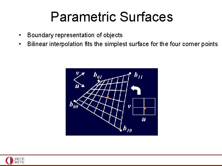
Parametric Surfaces • Boundary representation of objects • Bilinear interpolation fits the simplest surface for the four corner points

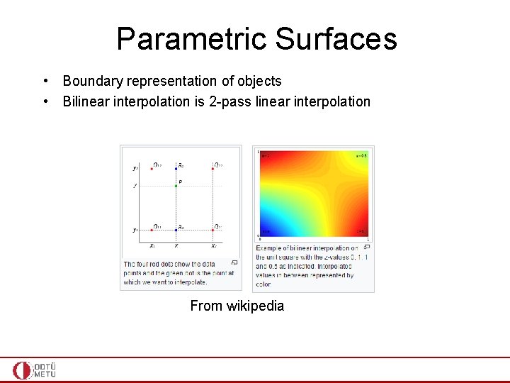
Parametric Surfaces • Boundary representation of objects • Bilinear interpolation is 2 -pass linear interpolation From wikipedia

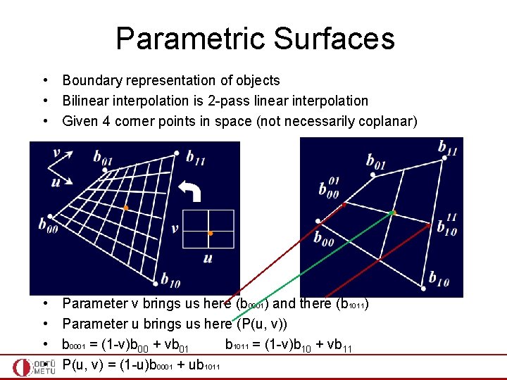
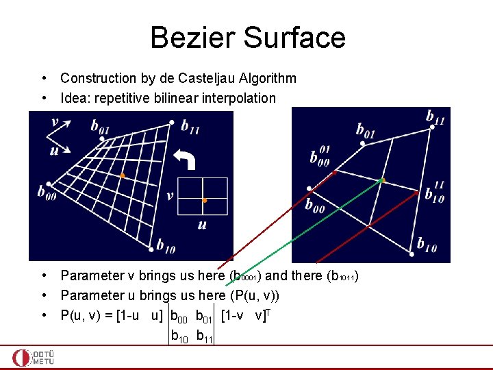
Parametric Surfaces • Boundary representation of objects • Bilinear interpolation is 2 -pass linear interpolation • Given 4 corner points in space (not necessarily coplanar) • • Parameter v brings us here (b 0001) and there (b 1011) Parameter u brings us here (P(u, v)) b 0001 = (1 -v)b 00 + vb 01 b 1011 = (1 -v)b 10 + vb 11 P(u, v) = (1 -u)b 0001 + ub 1011

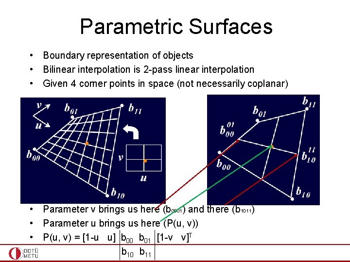
Parametric Surfaces • Boundary representation of objects • Bilinear interpolation is 2 -pass linear interpolation • Given 4 corner points in space (not necessarily coplanar) • Parameter v brings us here (b 0001) and there (b 1011) • Parameter u brings us here (P(u, v)) • P(u, v) = [1 -u u] b 00 b 01 [1 -v v]T b 10 b 11

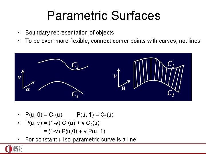
Parametric Surfaces • Boundary representation of objects • To be even more flexible, connect corner points with curves, not lines • P(u, 0) = C 1(u) P(u, 1) = C 2(u) • P(u, v) = (1 -v) C 1(u) + v C 2(u) = (1 -v) P(u, 0) + v P(u, 1) • For constant u iso-parametric curve is a line

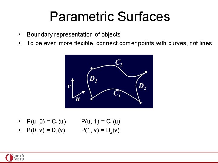
Parametric Surfaces • Boundary representation of objects • To be even more flexible, connect corner points with curves, not lines • P(u, 0) = C 1(u) • P(0, v) = D 1(v) P(u, 1) = C 2(u) P(1, v) = D 2(v)

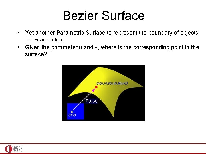
Bezier Surface • Yet another Parametric Surface to represent the boundary of objects – Bezier surface • Given the parameter u and v, where is the corresponding point in the surface?

Bezier Curve (Revisit) • Construction by de Casteljau Algorithm • Idea: repetitive linear interpolation • P 01(u) = (1 -u)P 0 + u. P 11(u) = (1 -u)P 1 + u. P 2 • P 02(u) = (1 -u)P 01(u) + u. P 11(u) = (1 -u)2 P 0 + 2 u(1 -u)P 1 + u 2 P 2

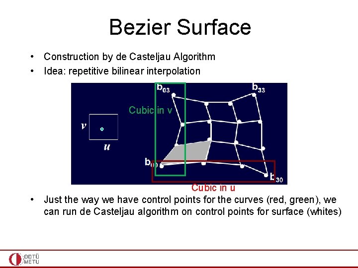
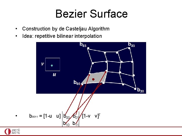
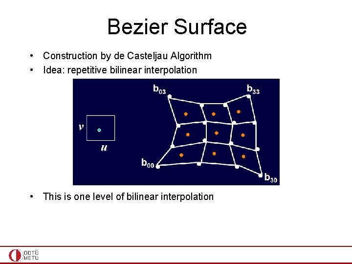
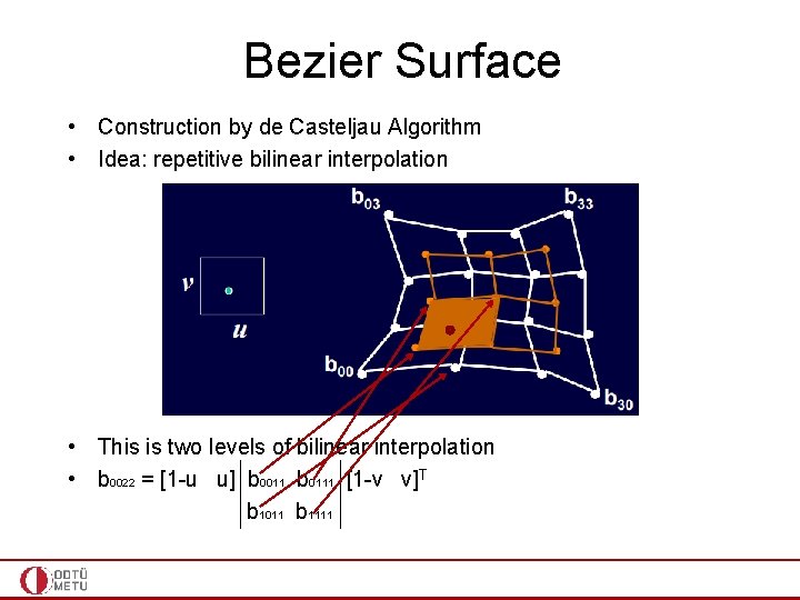
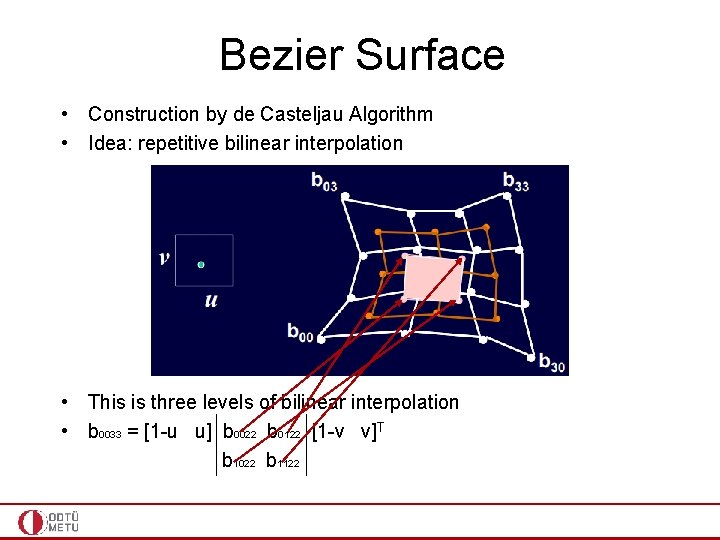
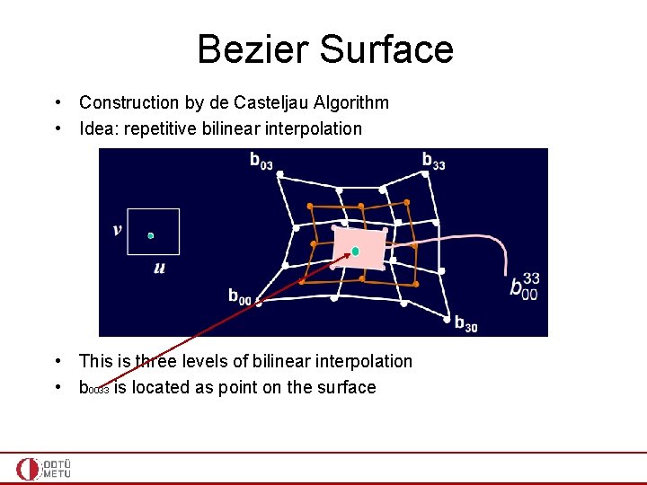
Bezier Surface • Construction by de Casteljau Algorithm • Idea: repetitive bilinear interpolation Cubic in v Cubic in u • Just the way we have control points for the curves (red, green), we can run de Casteljau algorithm on control points for surface (whites)

Bezier Surface • Construction by de Casteljau Algorithm • Idea: repetitive bilinear interpolation • Parameter v brings us here (b 0001) and there (b 1011) • Parameter u brings us here (P(u, v)) • P(u, v) = [1 -u u] b 00 b 01 [1 -v v]T b 10 b 11

Bezier Surface • Construction by de Casteljau Algorithm • Idea: repetitive bilinear interpolation • b 0011 = [1 -u u] b 00 b 01 [1 -v v]T b 10 b 11

Bezier Surface • Construction by de Casteljau Algorithm • Idea: repetitive bilinear interpolation • This is one level of bilinear interpolation

Bezier Surface • Construction by de Casteljau Algorithm • Idea: repetitive bilinear interpolation • This is two levels of bilinear interpolation • b 0022 = [1 -u u] b 0011 b 0111 [1 -v v]T b 1011 b 1111

Bezier Surface • Construction by de Casteljau Algorithm • Idea: repetitive bilinear interpolation • This is three levels of bilinear interpolation • b 0033 = [1 -u u] b 0022 b 0122 [1 -v v]T b 1022 b 1122

Bezier Surface • Construction by de Casteljau Algorithm • Idea: repetitive bilinear interpolation • This is three levels of bilinear interpolation • b 0033 is located as point on the surface

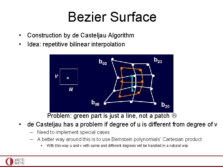
Bezier Surface • Construction by de Casteljau Algorithm • Idea: repetitive bilinear interpolation Problem: green part is just a line, not a patch • de Casteljau has a problem if degree of u is different from degree of v – Need to implement special cases – A better way around this is to use Bernstein polynomials’ Cartesian product • With this way u and v with same and different degrees will be handled in a natural way

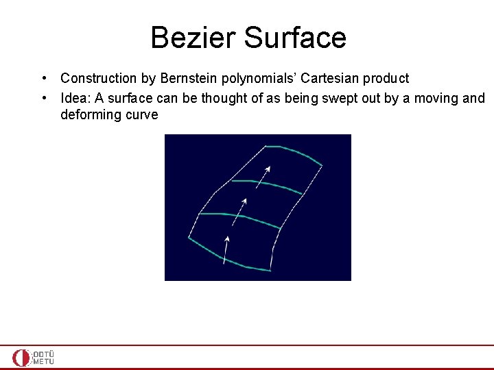
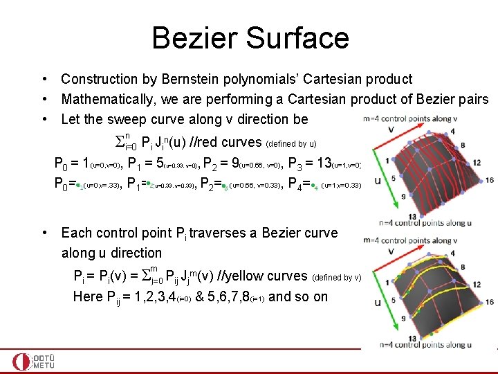
Bezier Surface • Construction by Bernstein polynomials’ Cartesian product • Idea: A surface can be thought of as being swept out by a moving and deforming curve

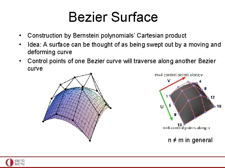
Bezier Surface • Construction by Bernstein polynomials’ Cartesian product • Idea: A surface can be thought of as being swept out by a moving and deforming curve • Control points of one Bezier curve will traverse along another Bezier curve n ≠ m in general

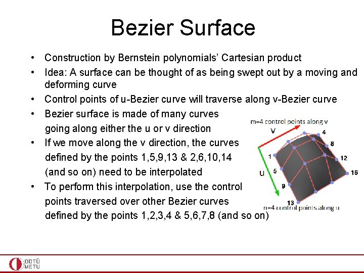
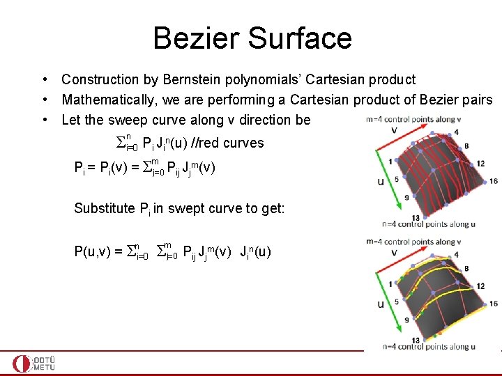
Bezier Surface • Construction by Bernstein polynomials’ Cartesian product • Idea: A surface can be thought of as being swept out by a moving and deforming curve • Control points of u-Bezier curve will traverse along v-Bezier curve • Bezier surface is made of many curves going along either the u or v direction • If we move along the v direction, the curves defined by the points 1, 5, 9, 13 & 2, 6, 10, 14 (and so on) need to be interpolated • To perform this interpolation, use the control points traversed over other Bezier curves defined by the points 1, 2, 3, 4 & 5, 6, 7, 8 (and so on)

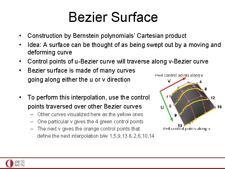
Bezier Surface • Construction by Bernstein polynomials’ Cartesian product • Idea: A surface can be thought of as being swept out by a moving and deforming curve • Control points of u-Bezier curve will traverse along v-Bezier curve • Bezier surface is made of many curves going along either the u or v direction • To perform this interpolation, use the control points traversed over other Bezier curves – Other curves visualized here as the yellow ones – One particular v gives the 4 green control points – The next v gives the orange control points that define the next interpolation b/w 1, 5, 9, 13 & 2, 6, 10, 14

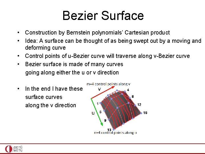
Bezier Surface • Construction by Bernstein polynomials’ Cartesian product • Idea: A surface can be thought of as being swept out by a moving and deforming curve • Control points of u-Bezier curve will traverse along v-Bezier curve • Bezier surface is made of many curves going along either the u or v direction • In the end I have these surface curves along the v direction

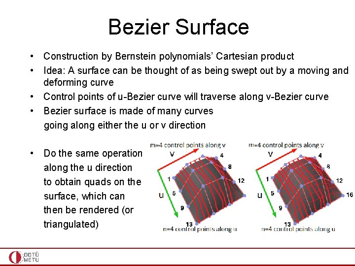
Bezier Surface • Construction by Bernstein polynomials’ Cartesian product • Idea: A surface can be thought of as being swept out by a moving and deforming curve • Control points of u-Bezier curve will traverse along v-Bezier curve • Bezier surface is made of many curves going along either the u or v direction • Do the same operation along the u direction to obtain quads on the surface, which can then be rendered (or triangulated)

Bezier Surface • Construction by Bernstein polynomials’ Cartesian product • Mathematically, we are performing a Cartesian product of Bezier pairs • Let the sweep curve along v direction be n Σi=0 Pi Jin(u) //red curves (defined by u) P 0 = 1(u=0, v=0), P 1 = 5 P 0= (u=0, v=. 33), P 1= , P 2 = 9(u=0. 66, v=0), P 3 = 13(u=1, v=0) , P 2= (u=0. 66, v=0. 33), P 4= (u=1, v=0. 33) (u=0. 33, v=0. 33) • Each control point Pi traverses a Bezier curve along u direction m Pi = Pi(v) = Σj=0 Pij Jjm(v) //yellow curves (defined by v) Here Pij = 1, 2, 3, 4(i=0) & 5, 6, 7, 8(i=1) and so on

Bezier Surface • Construction by Bernstein polynomials’ Cartesian product • Mathematically, we are performing a Cartesian product of Bezier pairs • Let the sweep curve along v direction be n Σi=0 Pi Jin(u) //red curves m Pi = Pi(v) = Σj=0 Pij Jjm(v) Substitute Pi in swept curve to get: P(u, v) = Σni=0 Σmj=0 Pij Jjm(v) Jin(u)

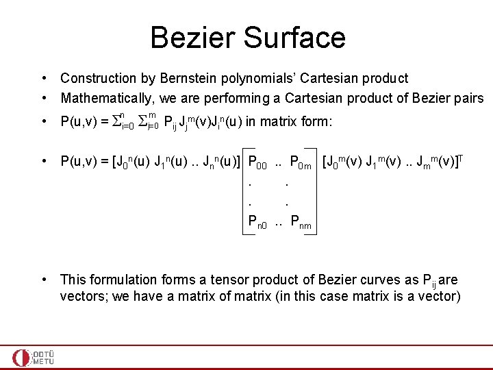
Bezier Surface • Construction by Bernstein polynomials’ Cartesian product • Mathematically, we are performing a Cartesian product of Bezier pairs n m • P(u, v) = Σi=0 Σj=0 Pij Jjm(v)Jin(u) in matrix form: • P(u, v) = [J 0 n(u) J 1 n(u). . Jnn(u)] P 00. . P 0 m [J 0 m(v) J 1 m(v). . Jmm(v)]T. . Pn 0. . Pnm • This formulation forms a tensor product of Bezier curves as Pij are vectors; we have a matrix of matrix (in this case matrix is a vector)

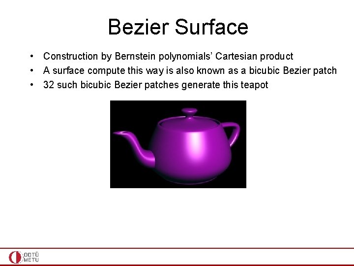
Bezier Surface • Construction by Bernstein polynomials’ Cartesian product • A surface compute this way is also known as a bicubic Bezier patch • 32 such bicubic Bezier patches generate this teapot