CENG 477 Introduction to Computer Graphics Rasterization Goal

CENG 477 Introduction to Computer Graphics Rasterization

Goal • After projection transformations we have a 2 D scene in our viewport • Convert 2 D scene (continuous) to pixels/rasters of the display device (discrete) • We refer this process as – Rasterization, or – Pixelization, or – Scan conversion • We will look at rasterization process in terms of drawing algorithms for various primitives

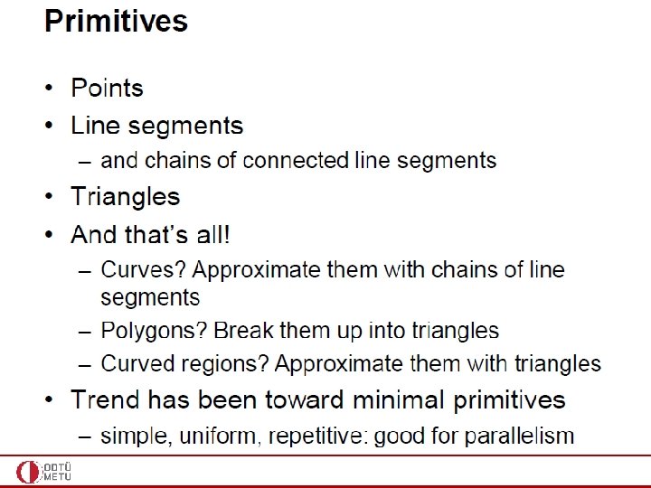
Primitives • Graphic SW and HW provide subroutines to describe a scene in terms of basic geometric structures called output primitives. • Output primitives are combined to form complex structures • Simplest primitives – Point (pixel) – Line segment

Rasterization • Converting output primitives into frame buffer updates. Choose which pixels contain which intensity value. • Constraints – Straight lines should appear as a straight line – primitives should start and end accurately – Primitives should have a consistent brightness along their length – They should be drawn rapidly

Line Drawing Algorithms • Slope-intercept line equation

Line Drawing Algorithms • Simple approach: sample a line at discrete positions at one coordinate from start point to end point, calculate the other coordinate value from line equation (slope-intercept line equation). Is this correct? • If m>1, increment y uniformly and find x If m≤ 1, increment x uniformly and find y //exchange the role of x and y

x 0=. 5, y 0=1. 91+. 37/2 = 2. 09 x 1 2 3 4 5 6 y 2. 28 2. 65 3. 02 3. 39 3. 76 4. 13

Plotted pixels • Digitize the line with endpoints (20, 10) and (30, 18) 18 x 20 21 22 23 24 25 26 27 28 29 30 10 20 21 22 25 30 y 10 10. 8 11. 6 12. 4 13. 2 14 14. 8 15. 6 16. 4 17. 2 18

Digital Differential Analyzer • Simple approach: too many floating point operations and repeated calculations • Calculate from for a value

d = ynew – y for the initialization

Suppose m=. 3. 3. 6 (>. 5) -. 1 y y+1 . 2 y+1 . 5 y+1 . 8 y+2 . 1 y+2 . 4 y+2

DDA Algorithm y = 1. 91 +. 37 x x 0=. 5, y 0=1. 91+. 37/2 = 2. 09 x 1 2 3 4 5 6 y 2 3 3 3 4 4 d 2. 65 – 2 =. 65 – 1 +. 37 =. 02 +. 37 =. 39 +. 37 =. 76 – 1 +. 37 =. 13 +. 37 =. 5

DDA • Is faster than directly implementing y=mx+b. No floating point multiplications. We have floating point additions only at each step. • But what about round-off errors? • Can we get rid of floating point operations completely? • Yes – Midpoint Line Algorithm – Bresenham’s Line Algorithm • Both produce the same exact result (for lines and integer circles, the midpoint formulation reduces to the Bresenham formulation) • Both can be extended to other primitives such as circle • We study the former as it is easier to understand

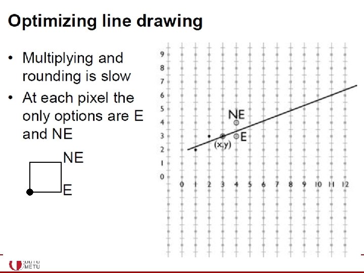
DDA • Is faster than directly implementing y=mx+b. No floating point multiplications. We have floating point additions only at each step. • But what about round-off errors? • Can we get rid of floating point operations completely? • Yes – Midpoint Line Algorithm • Idea: Find out if the midpoint b/w E-NE pixels is above or below the ideal line – Bresenham’s Line Algorithm • Idea: Choose the pixel closest to the ideal line

Midpoint Line Algorithm • Again assume lines with slopes in [0, 1] interval • Simply exchange the role of x and y for other lines

Midpoint Line Algorithm • Decision based on the midpoint of the two candidate pixels, namely E and NE • Find on what side of the line the midpoint M is • If below, NE is closer to the line (choose NE) • If above, E is closer to the line (choose E)

Midpoint Line Algorithm • • F(x, y) = 0 (x, y) on line F(x, y) < 0 (x, y) below line F(x, y) > 0 (x, y) above line What is F? observe the sign as you go in this direction

Midpoint Line Algorithm • • Implicit line equation y = mx + b y - mx – b = 0 y – dy/dx x – b = 0 dy x – dx y + dx b = 0 • F(x, y) = ax + by + c = 0 • Hence, a = dy, b = -dx, c = b dx

Midpoint Line Algorithm • F(x, y) = ax + by + c = 0 • Hence, a = dy, b = -dx, c = b dx • F(M) = F(xp + 1, yp + 1/2) = d • d = a(xp+1) + b(yp+1/2) + c • If d > 0, M is above the line, choose E • If d < 0, M is below the line, choose NE (xp, yp)

Midpoint Line Algorithm • Now we decided on E or NE; how do we change d’s? • According to this decision consider further M’ or M’’ • • • If we have plotted/decided E, consider M’ dnew = F(M’) = F(xp + 2, yp + 1/2) dnew = a(xp + 2) + b(yp + 1/2) + c dold = F(M) = a(xp + 1) + b(yp + 1/2) + c dd. E = dnew - dold = a = dy //delta d when E is selected When const dy added to dold I get the desired dnew quickly

Midpoint Line Algorithm • Now we decided on E or NE; how do we change d’s? • According to this decision consider further M’ or M’’ • • • If we have plotted/decided NE, consider M’’ dnew = F(M’’) = F(xp + 2, yp + 3/2) dnew = a(xp + 2) + b(yp + 3/2) + c dold = F(M) = a(xp + 1) + b(yp + 1/2) + c dd. NE = dnew - dold = a + b = dy-dx //delta d when NE selected When const dy-dx added to dold I get the desired dnew quickly

Midpoint Line Algorithm • Everything* ready to give the full algo • Need to eliminate division to stay completely in integer arithmetic • • • Consider the decision variable at the starting case dstart = F(x 0 + 1, y 0+1/2) = a(x 0 + 1) + b(y 0+1/2) + c dstart = ax 0 + by 0 + c + a + b/2 dstart = 0 + a + b/2 //’cos (x 0, y 0) on the line dstart = a + b/2 = dy – dx/2 //division Solution: use F(x, y) = 2(ax + by + c) – Note that this trick does not affect 0, -ve, +ve output structure of F

Midpoint Line Algorithm • Complete Algorithm (no floating ops) dx=x 1 -x 0; dy=y 1 -y 0; d=2 dy-dx; dd. E = 2 dy; dd. NE = 2(dy-dx); x=x 1; y=y 1; output(x, y); while (x<x 1) if d < 0 d += dd. NE; x++; y++; else d += dd. E; x++; output(x, y);

Float vs Integer • The midpoint algorithm was originally developed by Pitteway in 1967 • Floating point arithmetic was very expensive at the time • Does it still matter? • We implemented both algorithms and drew one million lines each between 1000 and 1400 pixels long: – – – Test run on Intel Core i 7 CPU at 3. 2 GHz Compiled with g++ and –O 2 option Basic algorithm: 7. 2 seconds Optimized algorithm: 3 seconds So it still makes a difference! CENG 477 - Computer Graphics 26

Example • Using Midpoint Line Algorithm digitize the line with endpoints (20, 10) and (30, 18)

Example continued. . . 18 10 20 21 22 25 30

Plotted pixels 18 10 20 21 22 25 30

Bresenham's Line Algorithm • Same output as Midpoint Line Algorithm but different idea • Choose the pixel closest to the ideal line (not by midpoint) y=mx+b yk+1 dupper yk dlower xk xk+1 xk+2 xk+3

at step k+1: 0 if pk was negative 1 if pk was positive to calculate p 0 at the starting pixel position (x 0, y 0)

Bresenham’s Line-Drawing Algorithm

Midpoint Circle Algorithm • Drawing circle with a DDA-based approach is uncool – Due to the uneven spacing of nonlinear circle equation: x 2 + y 2 = R 2 – Run through x values, compute and round y //uncool

Midpoint Circle Algorithm • Break down the problem into octants • Assume 2 nd octant as I can recover correspondences on other octants using 8 -way symmetry

Midpoint Circle Algorithm • Decision based on the midpoint of the two candidate pixels, namely E and SE //assuming 2 nd octant • Find on what side of the circle the midpoint M is • F(x, y) = 0 (x, y) on circle • F(x, y) < 0 (x, y) in circle • F(x, y) > 0 (x, y) out circle • F(x, y) = x 2 + y 2 - R 2

Midpoint Circle Algorithm • Decision based on the midpoint of the two candidate pixels, namely E and SE //assuming 2 nd octant • Find on what side of the circle the midpoint M is • If in, E is closer to the circle (choose E) • If out, SE is closer to the circle (choose SE)

Midpoint Circle Algorithm • Now we decided on E or SE ; how do we change d’s? • According to this decision consider further ME or MSE • • • If we have decided E, consider ME dnew = F(ME) = F(xp + 2, yp - 1/2) dnew = (xp + 2)2 + (yp - 1/2)2 - R 2 dold = F(M) = F(xp + 1, yp - 1/2) = (xp + 1)2 + (yp - 1/2)2 - R 2 dd. E = dnew - dold = 2 xp + 3 //delta d when E selected When const 2 xp+3 added to dold I get desired dnew quickly

Midpoint Circle Algorithm • Now we decided on E or SE ; how do we change d’s? • According to this decision consider further ME or MSE • • • If we have decided SE, consider MSE dnew = F(ME) = F(xp + 2, yp - 3/2) dnew = (xp + 2)2 + (yp - 3/2)2 - R 2 dold = F(M) = F(xp + 1, yp - 1/2) = (xp + 1)2 + (yp - 1/2)2 - R 2 dd. SE = dnew - dold = 2 xp - 2 yp + 5//delta d when SE selected When const above added to dold I get desired dnew quickly

Midpoint Circle Algorithm • Everything* ready to give the full algo • • • Consider the decision variable at the starting case (0, R) start point //2 nd octant Next midpoint: (1, R – 1/2) dstart = F(1, R – 1/2) = 5/4 – R //has floating number Solution: think something similar to line case (slide 41) – A big deal as GPUs nowadays have float arithmetic built-in? Slide 26

Midpoint Circle Algorithm • Complete Algorithm x=0; y=R; d=5/4 – R; output(x, y); while (y>x) //in 2 nd octant if d < 0 d += 2 x+3; x++; //E else d += 2 x-2 y+5; x++; y--; //SE output(x, y);

Midpoint Circle Algorithm • Complete Algorithm (no floating ops) x=0; y=R; D=1 - R; //replace all d by D = d - ¼ //because increments are always integer, D< - ¼ <==> D<0 output(x, y); while (y>x) //in 2 nd octant if D < 0 D += 2 x+1; x++; //E else D += 2 x-2 y+2; x++; y--; //SE output(x, y);

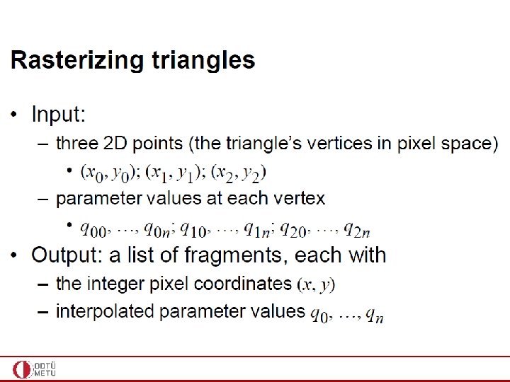
Rasterizing Triangles • Can’t we just draw each edge of the triangle (polygon) using DDA or Midpoint Line Algorithm? – We get a wireframe model then – We do not get the feeling of the area; coloring would help • We are looking for a drawing algorithm where we can fill the triangles with some color – Aka scan conversion of the triangle (polygon)

Rasterizing Triangles • Focus on triangles only because every polygon can be decomposed into triangles

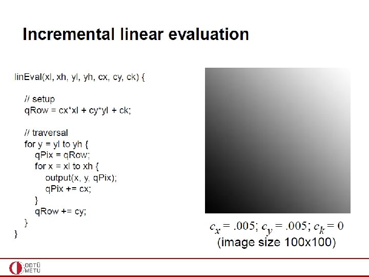
Scanning through the bounding box of the triangle, hence the name scan conversion

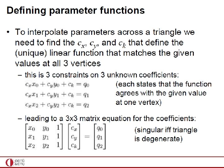
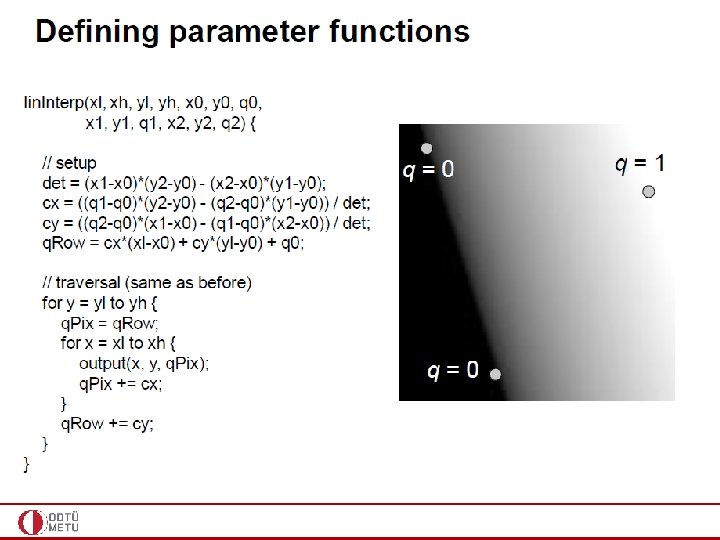
ck = q 0

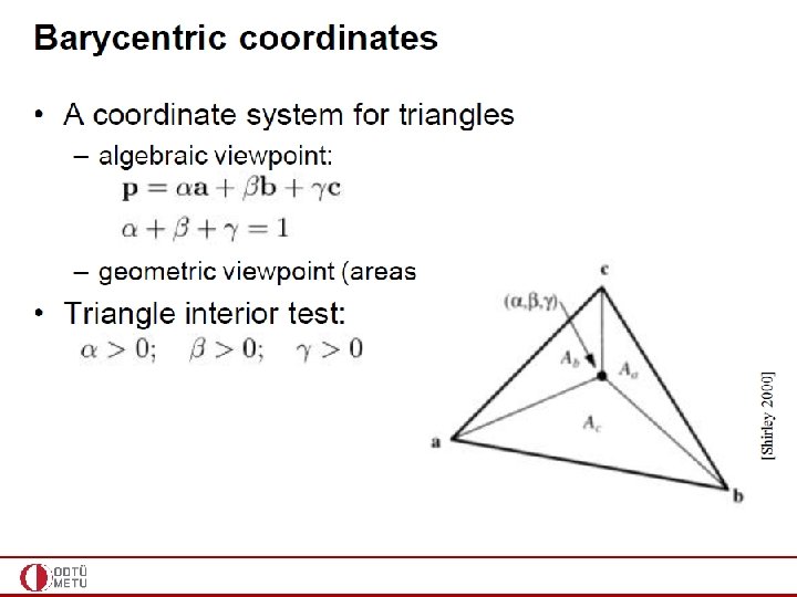
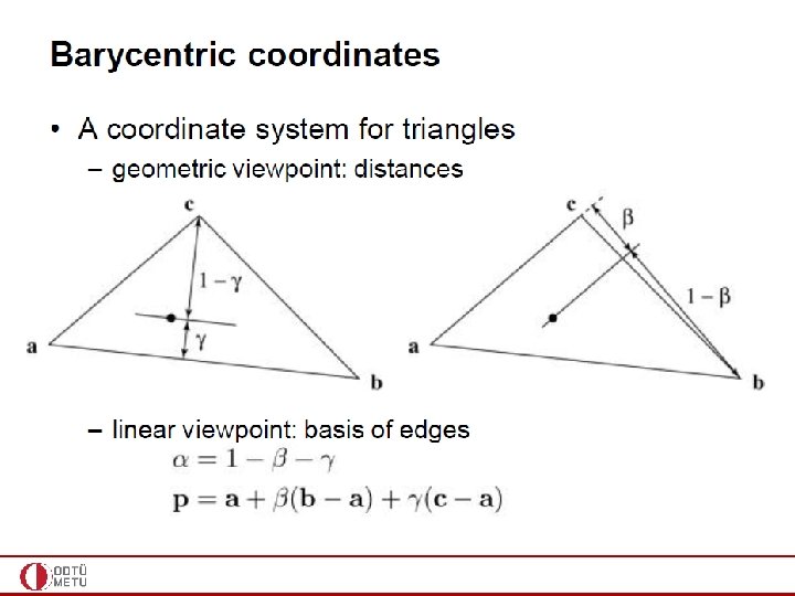
Computing the Barycentric Coordinates

Computing the Barycentric Coordinates (more efficient)

More clear view of the prev. eqs.

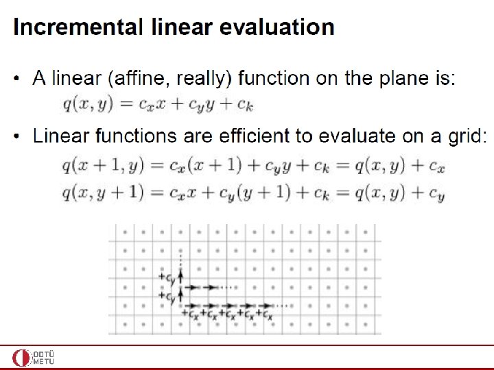
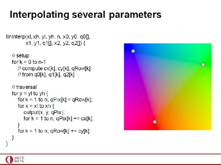
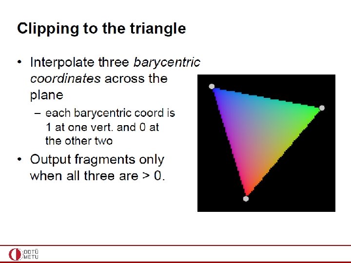
Triangle rasterization algorithm Combine this with incremental linear interpolation

Triangle Rasterization • Note that barycentric coordinates allow us to – Make the interior test //could have been done with line eq (slide 19) – Interpolate other attributes such as color: • So barycentric coordinates are the right way to go (x 1, y 1) (x 0, y 0) • Line equation based interior test: • For each pixel we visit, we must make an inside test with respect to all three edges • We can simply plug-in the (x, y) value of the visited pixel to each line equation • If all are negative, the pixel is inside the triangle (x 2, y 2) CENG 477 - Computer Graphics 59

More efficient than visiting bounding box pixels; here we use slope info to visit few

Fragment Processing • The previous stages of the pipeline (up to rasterization) is generally known as the vertex pipeline • Rasterization creates a set of fragments that make up the interior region of the primitive • The rest of the pipeline which operates on these fragments is called fragment pipeline • Fragment pipeline is comprised of several operations • The end result of fragment processing is the update of corresponding locations in the framebuffer CENG 477 - Computer Graphics 61

Fragment Processing Vertices Vertex Pipeline Fragment Pipeline Rasterization Framebuffer Color Buffer CENG 477 - Computer Graphics Depth Buffer Stencil Buffer 62

Fragment Processing • Fragment pipeline is comprised of many stages: – Following is Open. GL’s handling of the fragment pipeline – Different renderers may implement a different set of stages CENG 477 - Computer Graphics 63

Depth Buffer Test • Among these, the depth buffer test is very important to render primitives in correct order • Without depth buffer, the programmer must ensure to render primitives in a back to front order – Known as painter’s algorithm: From wikipedia. com CENG 477 - Computer Graphics 64

Depth Buffer Test • Binary space partitioning trees may be used for this purpose • However, they are costly to generate and may require splitting primitives due to impossible ordering cases: From wikipedia. com CENG 477 - Computer Graphics 65

Depth Buffer Test • When memory was a very valuable resource, such algorithms were implemented • Quake 3 was one of the main games that used painter’s algorithm using BSP trees • Each game level was stored as a huge BSP tree – Read more at: https: //www. bluesnews. com/abrash/chap 64. shtml CENG 477 - Computer Graphics 66

Depth Buffer Test • Main Idea: – At each pixel, keep track of the distance to the closest fragment that has been drawn in a separate buffer – Discard fragments that are further away than that distance – Otherwise, draw the fragment and update the z-buffer value with the z value of that fragment • Requires an extra memory region, called the depth buffer, to implement this solution • At the beginning of every frame, the depth buffer is reset to infinity (1. 0 f in practice if the depth range is [0. 0 f, 1. 0 f]) • Depth buffer is also known as z-buffer CENG 477 - Computer Graphics 67

Example Initial state of depth buffer z-values of the first triangle Resulting depth buffer z-values of the second triangle Resulting depth buffer wikipedia. com CENG 477 - Computer Graphics 68

Depth Range • The range of values written to the depth buffer can generally be controlled by the programmer • In Open. GL, the command gl. Depth. Range(z. Min, z. Max) is used • The default depth range is [0, 1] • The z-value in the canonical viewing volume (CVV), which is in range [-1, 1] is scaled to this range during the viewport transform • gl. Depth. Range is to the z-values what gl. Viewport(x, y, width, height) is to the xand y-values CENG 477 - Computer Graphics 69

Z-Fighting • Remember that the z-values get compressed to [0, 1] range from the [-n: -f] range after projection and viewport transforms • Observe how it looks for n = 10 and f = 50 CENG 477 – Computer Graphics 70

Z-Fighting • Remember that the z-values get compressed to [0, 1] range from the [-n: -f] range after projection and viewport transforms • Observe the same for n = 10 and f = 200 CENG 477 – Computer Graphics 71

Z-Fighting • With a limited precision depth buffer, fragments that are close in depth may get mapped to the same z-value CENG 477 – Computer Graphics 72

Z-Fighting • The compression is more severe for with larger depth range • This may cause a problem known as z-fighting: – Objects with originally different (but close) z-values get mapped to the same final z-value (due to limited precision) making it impossible to distinguish which one is in front and which one is behind CENG 477 – Computer Graphics 73

Z-Fighting • To avoid z-fighting, the depth range should be kept as small as possible for keeping the compression less severe • Alternatively, a floating point depth buffer can used – Unavailable in older hardware – Supported in all modern GPUs • Finally, the command gl. Polygon. Offset can be used to push and pull polygons a little to avoid z-fighting CENG 477 – Computer Graphics 74

Scissor Test • Scissor test is a per-fragment operation that discards fragments outside a certain rectangular region Scissor rectangle Without scissor Result In Open. GL, gl. Scissor command is used for this purpose Note that this operation is different from clipping CENG 477 - Computer Graphics 75

Stencil Test • While scissor test can be used to mask out rectangles, stencil test can be used to mask arbitrary fragments • Requires a different buffer known as the stencil buffer Original Stencil Buffer Result From research. ncl. ac. uk CENG 477 - Computer Graphics 76

Stencil Test • Typically depth and stencil buffers are combined to produce single buffer made of 24 -bit depth and 8 -bit stencil information for each pixel Pixel 1 Pixel 0 D S D S D S … … CENG 477 - Computer Graphics 77

Stencil Test • Stencil buffer and stencil test can also be used to implement one type of shadowing algorithms (we’ll learn this later) Doom 3 CENG 477 - Computer Graphics 78

Alpha Blending • Alpha blending is another fragment operation in which new objects can be blended with the existing contents of the color buffer for a variety of effects Without blending With blending CENG 477 - Computer Graphics 79

Summary • At the end of the pipeline, input vertices with connectivity information end of populating certain regions of the framebuffer • This pipeline can be implemented on the software (CPU), hardware (GPU) or both (CPU + GPU) Vertex Pipeline Fragment Pipeline Rasterization Framebuffer Vertices Color Buffer CENG 477 - Computer Graphics Depth Buffer Stencil Buffer 80