CENG 450 Computer Systems and Architecture Lecture 11

CENG 450 Computer Systems and Architecture Lecture 11 Amirali Baniasadi amirali@ece. uvic. ca 1

This Lecture z Branch Prediction z Multiple Issue 2

Branch Prediction z Predicting the outcome of a branch y Direction: x. Taken / Not Taken x. Direction predictors y Target Address x. PC+offset (Taken)/ PC+4 (Not Taken) x. Target address predictors • Branch Target Buffer (BTB) 3

Why do we need branch prediction? z Branch prediction y Increases the number of instructions available for the scheduler to issue. Increases instruction level parallelism (ILP) y Allows useful work to be completed while waiting for the branch to resolve 4

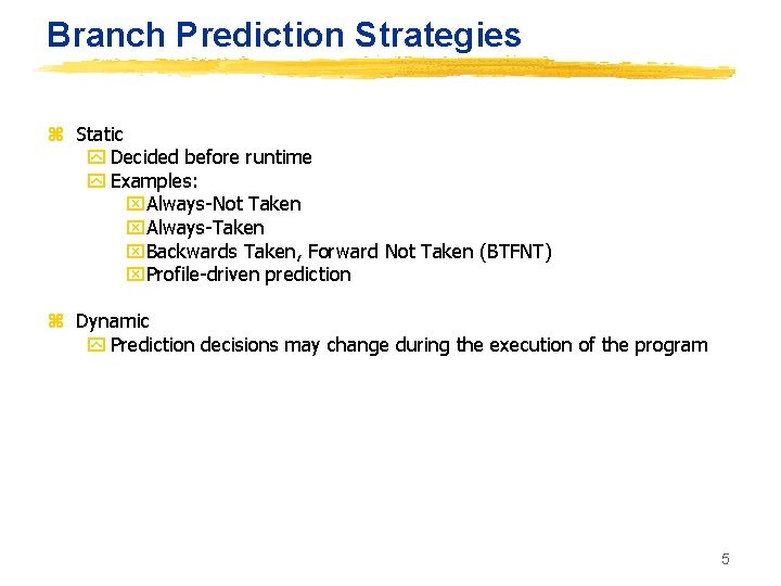
Branch Prediction Strategies z Static y Decided before runtime y Examples: x. Always-Not Taken x. Always-Taken x. Backwards Taken, Forward Not Taken (BTFNT) x. Profile-driven prediction z Dynamic y Prediction decisions may change during the execution of the program 5

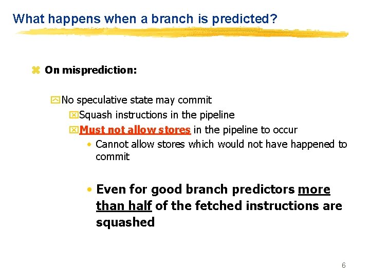
What happens when a branch is predicted? z On misprediction: y No speculative state may commit x. Squash instructions in the pipeline x. Must not allow stores in the pipeline to occur • Cannot allow stores which would not have happened to commit • Even for good branch predictors more than half of the fetched instructions are squashed 6

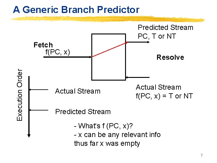
A Generic Branch Predictor Predicted Stream PC, T or NT Execution Order Fetch f(PC, x) Resolve Actual Stream f(PC, x) = T or NT Predicted Stream - What’s f (PC, x)? - x can be any relevant info thus far x was empty 7

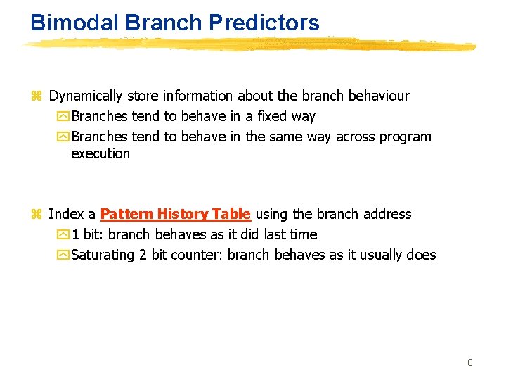
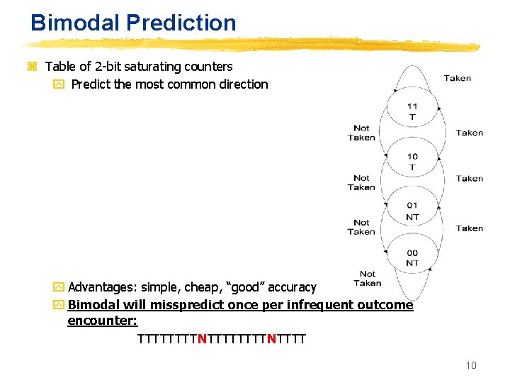
Bimodal Branch Predictors z Dynamically store information about the branch behaviour y Branches tend to behave in a fixed way y Branches tend to behave in the same way across program execution z Index a Pattern History Table using the branch address y 1 bit: branch behaves as it did last time y Saturating 2 bit counter: branch behaves as it usually does 8

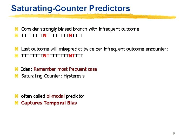
Saturating-Counter Predictors z Consider strongly biased branch with infrequent outcome z TTTTTTTTNTTTT z Last-outcome will misspredict twice per infrequent outcome encounter: z TTTTTTTTNTTTT z Idea: Remember most frequent case z Saturating-Counter: Hysteresis z often called bi-modal predictor z Captures Temporal Bias 9

Bimodal Prediction z Table of 2 -bit saturating counters y Predict the most common direction y Advantages: simple, cheap, “good” accuracy y Bimodal will misspredict once per infrequent outcome encounter: TTTTTTTTNTTTT 10

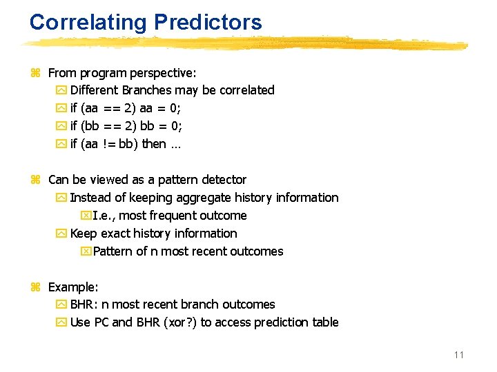
Correlating Predictors z From program perspective: y Different Branches may be correlated y if (aa == 2) aa = 0; y if (bb == 2) bb = 0; y if (aa != bb) then … z Can be viewed as a pattern detector y Instead of keeping aggregate history information x. I. e. , most frequent outcome y Keep exact history information x. Pattern of n most recent outcomes z Example: y BHR: n most recent branch outcomes y Use PC and BHR (xor? ) to access prediction table 11

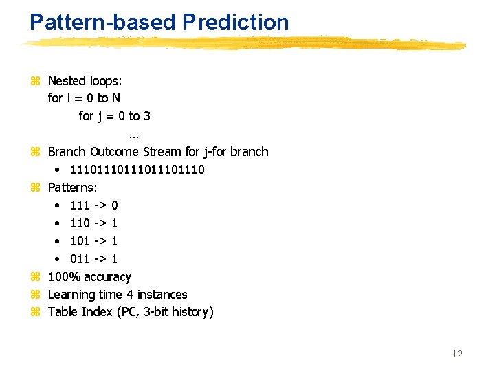
Pattern-based Prediction z Nested loops: for i = 0 to N for j = 0 to 3 … z Branch Outcome Stream for j-for branch • 111011101110 z Patterns: • 111 -> 0 • 110 -> 1 • 101 -> 1 • 011 -> 1 z 100% accuracy z Learning time 4 instances z Table Index (PC, 3 -bit history) 12

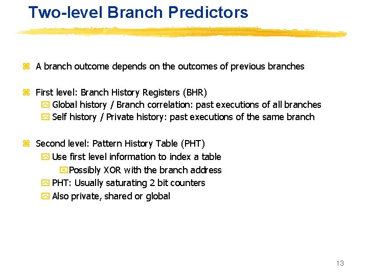
Two-level Branch Predictors z A branch outcome depends on the outcomes of previous branches z First level: Branch History Registers (BHR) y Global history / Branch correlation: past executions of all branches y Self history / Private history: past executions of the same branch z Second level: Pattern History Table (PHT) y Use first level information to index a table x. Possibly XOR with the branch address y PHT: Usually saturating 2 bit counters y Also private, shared or global 13

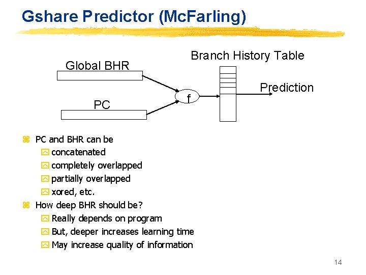
Gshare Predictor (Mc. Farling) Branch History Table Global BHR PC f Prediction z PC and BHR can be y concatenated y completely overlapped y partially overlapped y xored, etc. z How deep BHR should be? y Really depends on program y But, deeper increases learning time y May increase quality of information 14

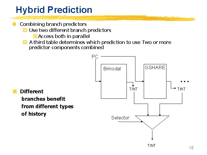
Hybrid Prediction z Combining branch predictors y Use two different branch predictors x Access both in parallel y A third table determines which prediction to use Two or more predictor components combined PC GSHARE Bimodal z Different branches benefit from different types of history . . . T/NT Selector T/NT 15

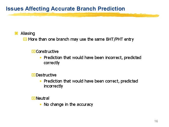
Issues Affecting Accurate Branch Prediction z Aliasing y More than one branch may use the same BHT/PHT entry x. Constructive • Prediction that would have been incorrect, predicted correctly x. Destructive • Prediction that would have been correct, predicted incorrectly x. Neutral • No change in the accuracy 16

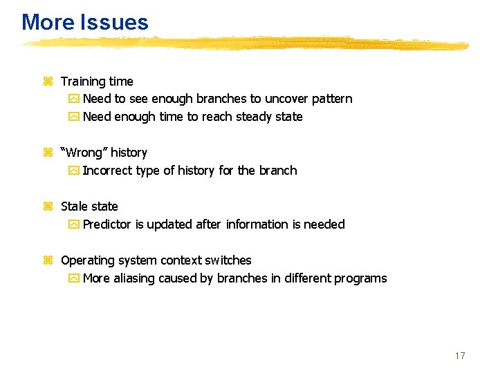
More Issues z Training time y Need to see enough branches to uncover pattern y Need enough time to reach steady state z “Wrong” history y Incorrect type of history for the branch z Stale state y Predictor is updated after information is needed z Operating system context switches y More aliasing caused by branches in different programs 17

Performance Metrics 8 Misprediction rate y Mispredicted branches per executed branch x. Unfortunately the most usually found 4 Instructions per mispredicted branch y Gives a better idea of the program behaviour x. Branches are not evenly spaced 18

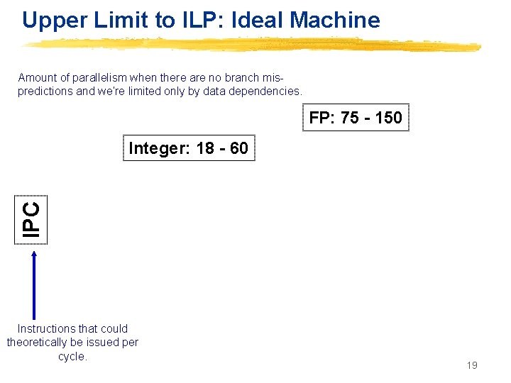
Upper Limit to ILP: Ideal Machine Amount of parallelism when there are no branch mispredictions and we’re limited only by data dependencies. FP: 75 - 150 IPC Integer: 18 - 60 Instructions that could theoretically be issued per cycle. 19

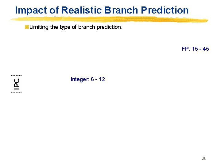
Impact of Realistic Branch Prediction z. Limiting the type of branch prediction. IPC FP: 15 - 45 Integer: 6 - 12 20

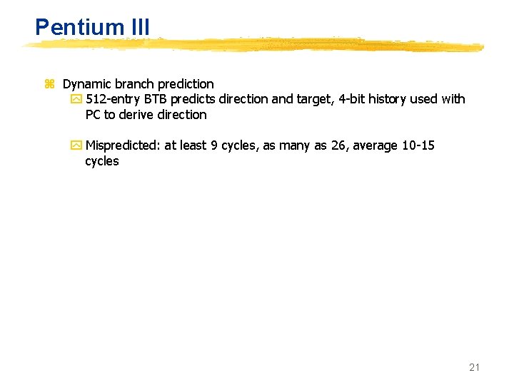
Pentium III z Dynamic branch prediction y 512 -entry BTB predicts direction and target, 4 -bit history used with PC to derive direction y Mispredicted: at least 9 cycles, as many as 26, average 10 -15 cycles 21

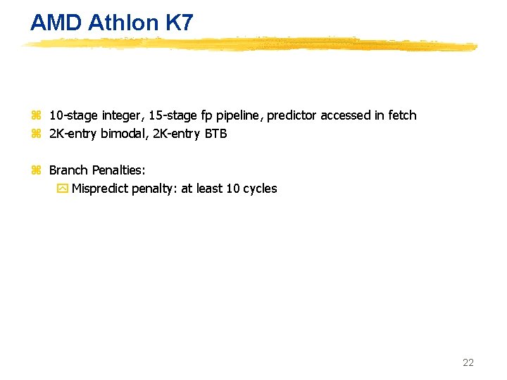
AMD Athlon K 7 z 10 -stage integer, 15 -stage fp pipeline, predictor accessed in fetch z 2 K-entry bimodal, 2 K-entry BTB z Branch Penalties: y Mispredict penalty: at least 10 cycles 22

Multiple Issue • Multiple Issue is the ability of the processor to start more than one instruction in a given cycle. • Superscalar processors • Very Long Instruction Word (VLIW) processors 23

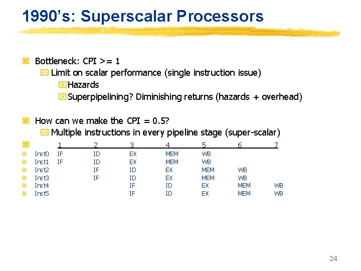
1990’s: Superscalar Processors z Bottleneck: CPI >= 1 y Limit on scalar performance (single instruction issue) x. Hazards x. Superpipelining? Diminishing returns (hazards + overhead) z How can we make the CPI = 0. 5? y Multiple instructions in every pipeline stage (super-scalar) z 1 2 3 4 5 6 7 z z z Inst 0 Inst 1 Inst 2 Inst 3 Inst 4 Inst 5 IF IF ID ID IF IF EX EX ID ID IF IF MEM EX EX ID ID WB WB MEM EX EX WB WB MEM WB WB 24

Superscalar Vs. VLIW z Religious debate, similar to RISC vs. CISC y Wisconsin + Michigan (Super scalar) Vs. Illinois (VLIW) y Q. Who can schedule code better, hardware or software? 25

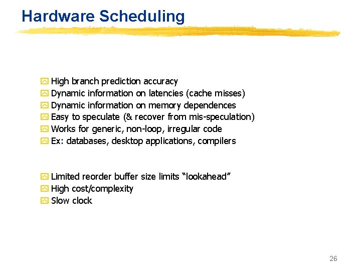
Hardware Scheduling y High branch prediction accuracy y Dynamic information on latencies (cache misses) y Dynamic information on memory dependences y Easy to speculate (& recover from mis-speculation) y Works for generic, non-loop, irregular code y Ex: databases, desktop applications, compilers y Limited reorder buffer size limits “lookahead” y High cost/complexity y Slow clock 26

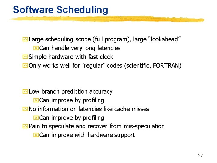
Software Scheduling y Large scheduling scope (full program), large “lookahead” x. Can handle very long latencies y Simple hardware with fast clock y Only works well for “regular” codes (scientific, FORTRAN) y Low branch prediction accuracy x. Can improve by profiling y No information on latencies like cache misses x. Can improve by profiling y Pain to speculate and recover from mis-speculation x. Can improve with hardware support 27

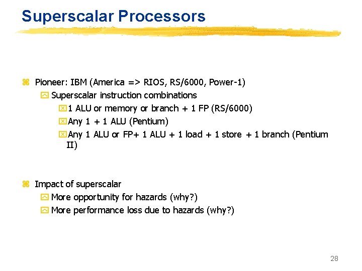
Superscalar Processors z Pioneer: IBM (America => RIOS, RS/6000, Power-1) y Superscalar instruction combinations x 1 ALU or memory or branch + 1 FP (RS/6000) x. Any 1 + 1 ALU (Pentium) x. Any 1 ALU or FP+ 1 ALU + 1 load + 1 store + 1 branch (Pentium II) z Impact of superscalar y More opportunity for hazards (why? ) y More performance loss due to hazards (why? ) 28

Superscalar Processors • Issues varying number of instructions per clock • Scheduling: Static (by the compiler) or dynamic(by the hardware) • Superscalar has a varying number of instructions/cycle (1 to 8), scheduled by compiler or by HW (Tomasulo). • IBM Power. PC, Sun Ultra. Sparc, DEC Alpha, HP 8000 29

Elements of Advanced Superscalars z High performance instruction fetching y Good dynamic branch and jump prediction y Multiple instructions per cycle, multiple branches per cycle? z Scheduling and hazard elimination y Dynamic scheduling y Not necessarily: Alpha 21064 & Pentium were statically scheduled y Register renaming to eliminate WAR and WAW z Parallel functional units, paths/buses/multiple register ports z High performance memory systems z Speculative execution 30

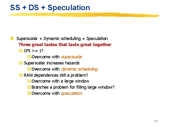
SS + DS + Speculation z Superscalar + Dynamic scheduling + Speculation Three great tastes that taste great together y CPI >= 1? x. Overcome with superscalar y Superscalar increases hazards x. Overcome with dynamic scheduling y RAW dependences still a problem? x. Overcome with a large window x. Branches a problem for filling large window? x. Overcome with speculation 31

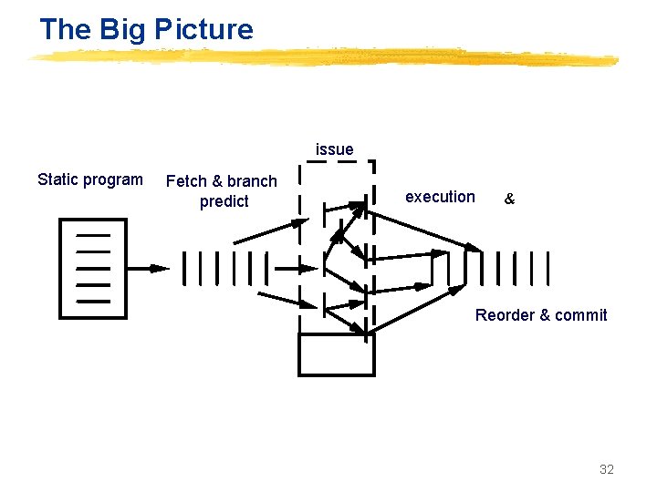
The Big Picture issue Static program Fetch & branch predict execution & Reorder & commit 32

Readings z New paper on branch prediction online. READ. z Material would be used in the THIRD quiz 33