CE 40763 Digital Signal Processing Fall 1992 LTI

CE 40763 Digital Signal Processing Fall 1992 LTI Systems Hossein Sameti Department of Computer Engineering Sharif University of Technology

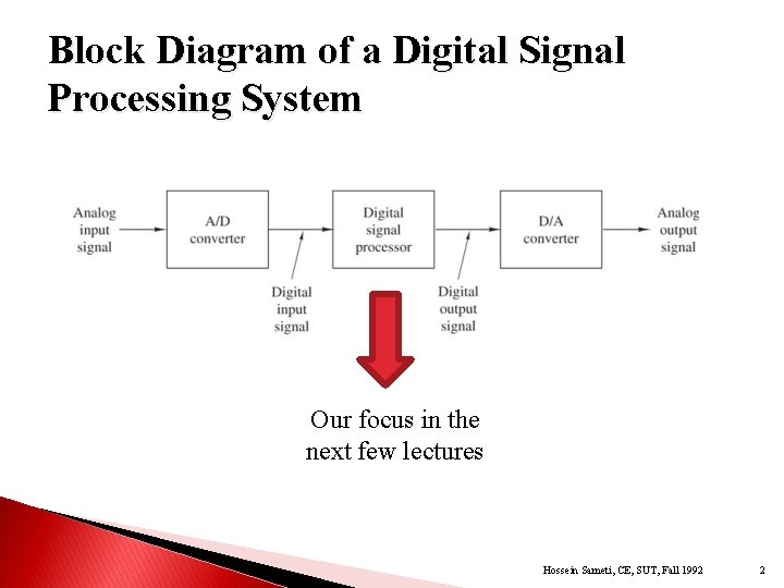
Block Diagram of a Digital Signal Processing System Our focus in the next few lectures Hossein Sameti, CE, SUT, Fall 1992 2

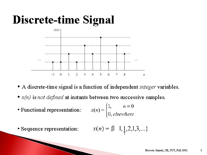
Discrete-time Signal • A discrete-time signal is a function of independent integer variables. • x(n) is not defined at instants between two successive samples. • Functional representation: • Sequence representation: Hossein Sameti, CE, SUT, Fall 1992 3

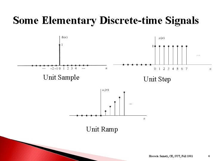
Some Elementary Discrete-time Signals Unit Sample Unit Step Unit Ramp Hossein Sameti, CE, SUT, Fall 1992 4

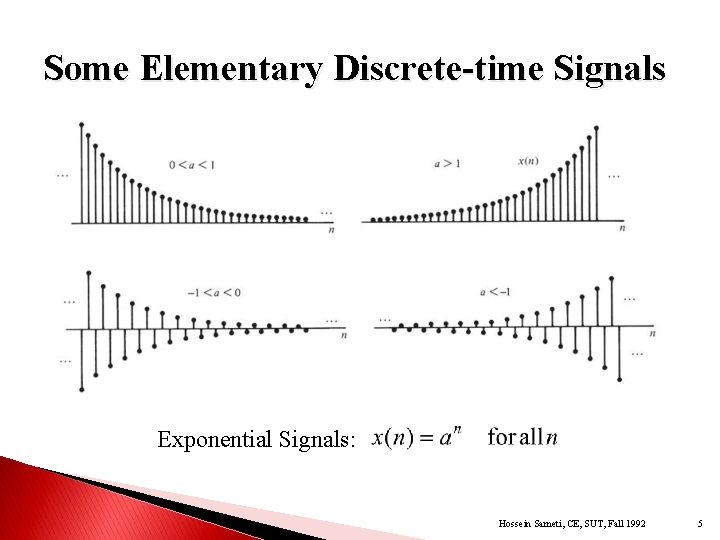
Some Elementary Discrete-time Signals Exponential Signals: Hossein Sameti, CE, SUT, Fall 1992 5

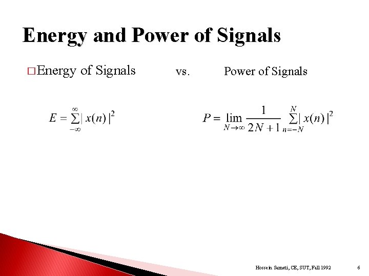
Energy and Power of Signals � Energy of Signals vs. Power of Signals Hossein Sameti, CE, SUT, Fall 1992 6

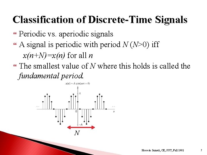
Classification of Discrete-Time Signals Periodic vs. aperiodic signals A signal is periodic with period N (N>0) iff x(n+N)=x(n) for all n The smallest value of N where this holds is called the fundamental period. N Hossein Sameti, CE, SUT, Fall 1992 7

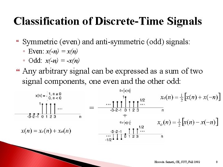
Classification of Discrete-Time Signals Symmetric (even) and anti-symmetric (odd) signals: ◦ Even: x(-n) = x(n) ◦ Odd: x(-n) = -x(n) Any arbitrary signal can be expressed as a sum of two signal components, one even and the other odd: = + Hossein Sameti, CE, SUT, Fall 1992 8

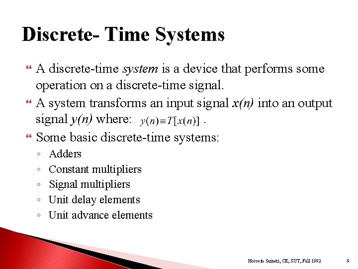
Discrete- Time Systems A discrete-time system is a device that performs some operation on a discrete-time signal. A system transforms an input signal x(n) into an output signal y(n) where: . Some basic discrete-time systems: ◦ ◦ ◦ Adders Constant multipliers Signal multipliers Unit delay elements Unit advance elements Hossein Sameti, CE, SUT, Fall 1992 9

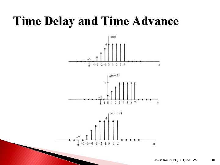
Time Delay and Time Advance Hossein Sameti, CE, SUT, Fall 1992 10

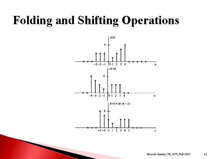
Folding and Shifting Operations Hossein Sameti, CE, SUT, Fall 1992 11

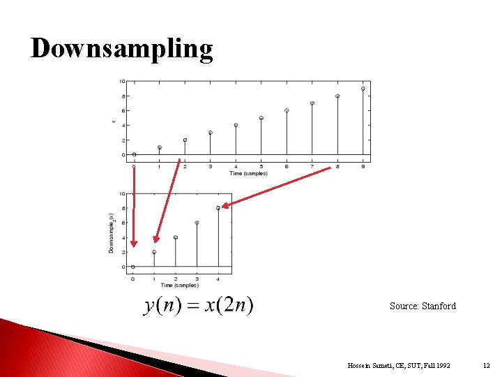
Downsampling Source: Stanford Hossein Sameti, CE, SUT, Fall 1992 12

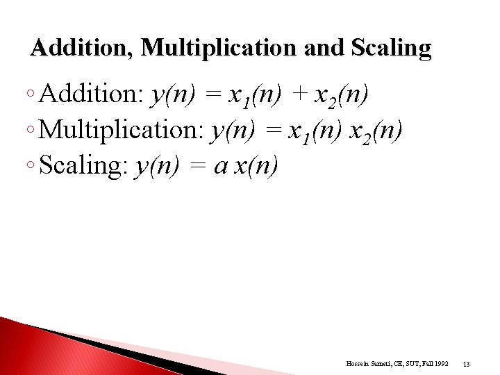
Addition, Multiplication and Scaling ◦ Addition: y(n) = x 1(n) + x 2(n) ◦ Multiplication: y(n) = x 1(n) x 2(n) ◦ Scaling: y(n) = a x(n) Hossein Sameti, CE, SUT, Fall 1992 13

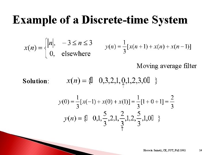
Example of a Discrete-time System Moving average filter Solution: Hossein Sameti, CE, SUT, Fall 1992 14

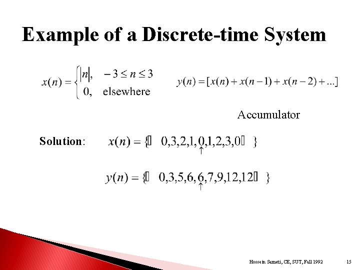
Example of a Discrete-time System Accumulator Solution: Hossein Sameti, CE, SUT, Fall 1992 15

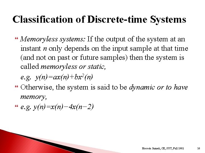
Classification of Discrete-time Systems Memoryless systems: If the output of the system at an instant n only depends on the input sample at that time (and not on past or future samples) then the system is called memoryless or static, e. g. y(n)=ax(n)+bx 2(n) Otherwise, the system is said to be dynamic or to have memory, e. g. y(n)=x(n)− 4 x(n− 2) Hossein Sameti, CE, SUT, Fall 1992 16

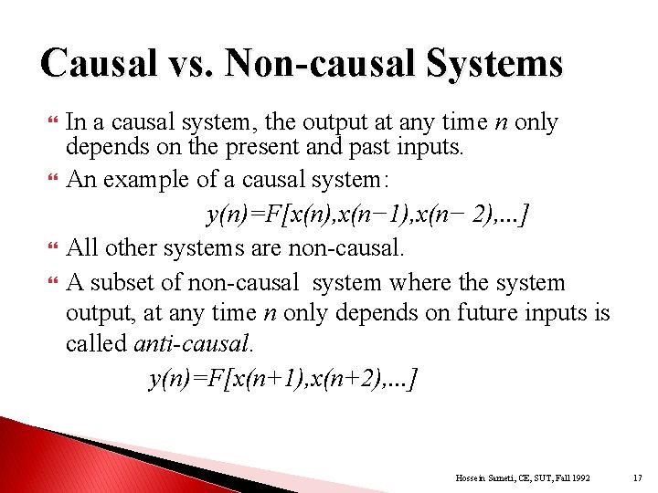
Causal vs. Non-causal Systems In a causal system, the output at any time n only depends on the present and past inputs. An example of a causal system: y(n)=F[x(n), x(n− 1), x(n− 2), . . . ] All other systems are non-causal. A subset of non-causal system where the system output, at any time n only depends on future inputs is called anti-causal. y(n)=F[x(n+1), x(n+2), . . . ] Hossein Sameti, CE, SUT, Fall 1992 17

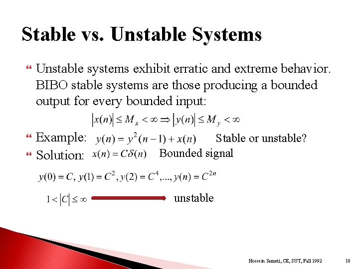
Stable vs. Unstable Systems Unstable systems exhibit erratic and extreme behavior. BIBO stable systems are those producing a bounded output for every bounded input: Example: Solution: Stable or unstable? Bounded signal unstable Hossein Sameti, CE, SUT, Fall 1992 18

Linear vs. Non-linear Systems Superposition principle: T[ax 1(n)+bx 2(n)]=a. T[x 1(n)]+b. T[x 2 (n)] A relaxed linear system with zero input produces a zero output. Scaling property Additivity property Hossein Sameti, CE, SUT, Fall 1992 19

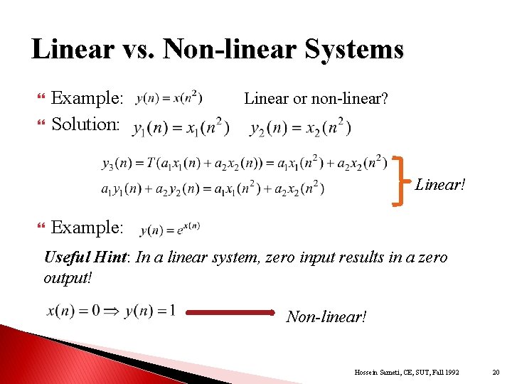
Linear vs. Non-linear Systems Example: Solution: Linear or non-linear? Linear! Example: Useful Hint: In a linear system, zero input results in a zero output! Non-linear! Hossein Sameti, CE, SUT, Fall 1992 20

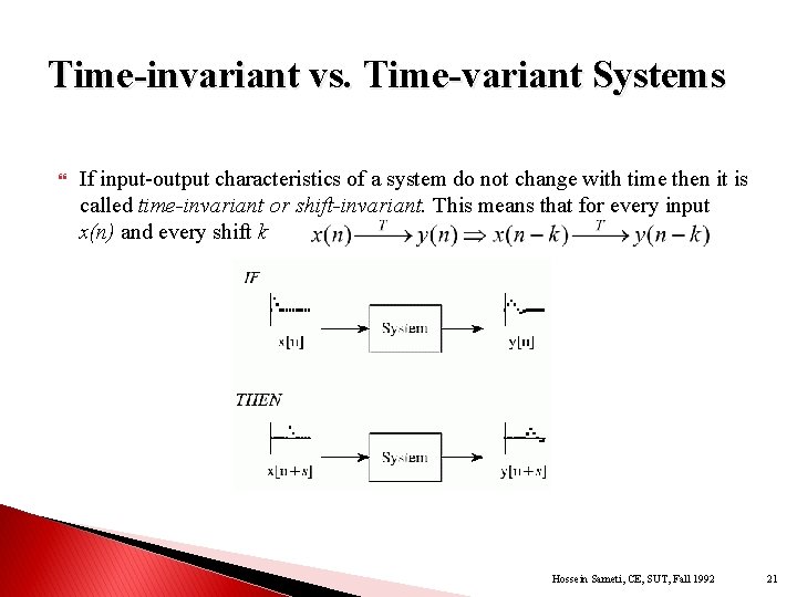
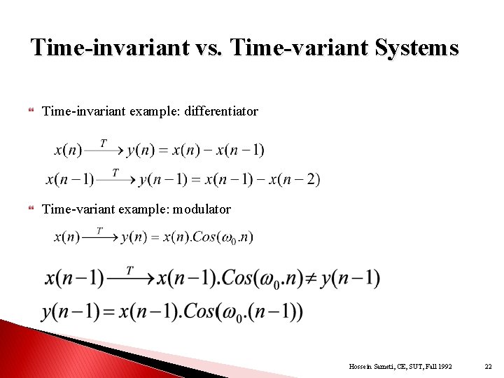
Time-invariant vs. Time-variant Systems If input-output characteristics of a system do not change with time then it is called time-invariant or shift-invariant. This means that for every input x(n) and every shift k Hossein Sameti, CE, SUT, Fall 1992 21

Time-invariant vs. Time-variant Systems Time-invariant example: differentiator Time-variant example: modulator Hossein Sameti, CE, SUT, Fall 1992 22

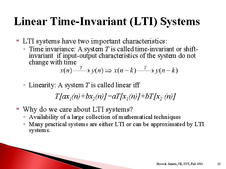
Linear Time-Invariant (LTI) Systems LTI systems have two important characteristics: ◦ Time invariance: A system T is called time-invariant or shiftinvariant if input-output characteristics of the system do not change with time ◦ Linearity: A system T is called linear iff T[ax 1(n)+bx 2(n)]=a. T[x 1(n)]+b. T[x 2 (n)] Why do we care about LTI systems? ◦ Availability of a large collection of mathematical techniques ◦ Many practical systems are either LTI or can be approximated by LTI systems. Hossein Sameti, CE, SUT, Fall 1992 23

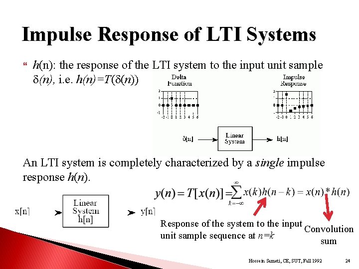
Impulse Response of LTI Systems h(n): the response of the LTI system to the input unit sample (n), i. e. h(n)=T( (n)) An LTI system is completely characterized by a single impulse response h(n). Response of the system to the input Convolution unit sample sequence at n=k sum Hossein Sameti, CE, SUT, Fall 1992 24

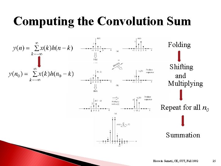
Computing the Convolution Sum Folding Shifting and Multiplying Repeat for all n 0 Summation Hossein Sameti, CE, SUT, Fall 1992 25

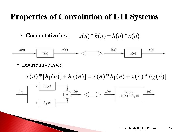
Properties of Convolution of LTI Systems • Commutative law: Distributive law: Hossein Sameti, CE, SUT, Fall 1992 26

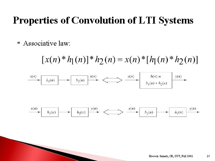
Properties of Convolution of LTI Systems Associative law: Hossein Sameti, CE, SUT, Fall 1992 27

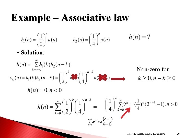
Example – Associative law • Solution: Non-zero for Hossein Sameti, CE, SUT, Fall 1992 28

Properties of LTI Systems

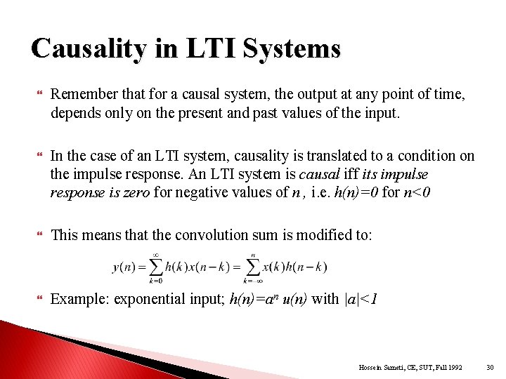
Causality in LTI Systems Remember that for a causal system, the output at any point of time, depends only on the present and past values of the input. In the case of an LTI system, causality is translated to a condition on the impulse response. An LTI system is causal iff its impulse response is zero for negative values of n , i. e. h(n)=0 for n<0 This means that the convolution sum is modified to: Example: exponential input; h(n)=an u(n) with |a|<1 Hossein Sameti, CE, SUT, Fall 1992 30

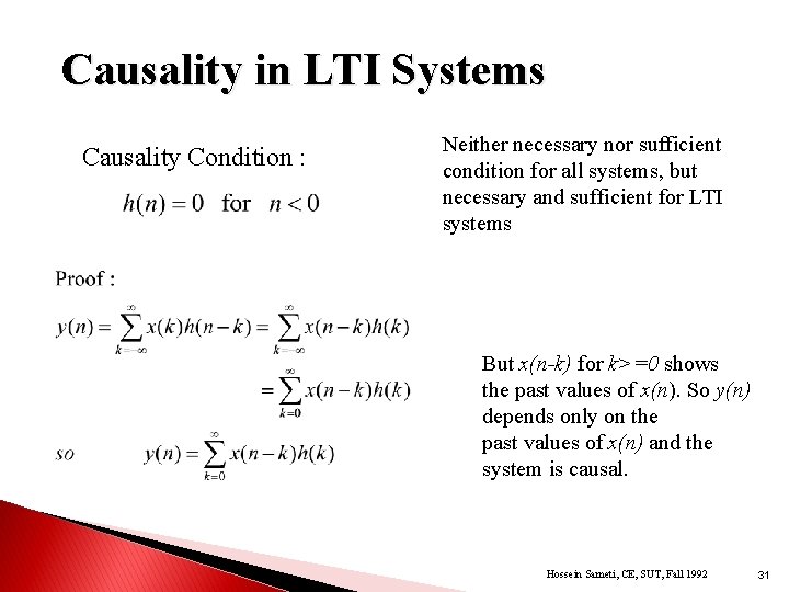
Causality in LTI Systems Causality Condition : Neither necessary nor sufficient condition for all systems, but necessary and sufficient for LTI systems But x(n-k) for k>=0 shows the past values of x(n). So y(n) depends only on the past values of x(n) and the system is causal. Hossein Sameti, CE, SUT, Fall 1992 31

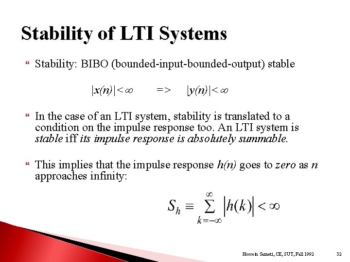
Stability of LTI Systems Stability: BIBO (bounded-input-bounded-output) stable |x(n)|< => |y(n)|< In the case of an LTI system, stability is translated to a condition on the impulse response too. An LTI system is stable iff its impulse response is absolutely summable. This implies that the impulse response h(n) goes to zero as n approaches infinity: Hossein Sameti, CE, SUT, Fall 1992 32

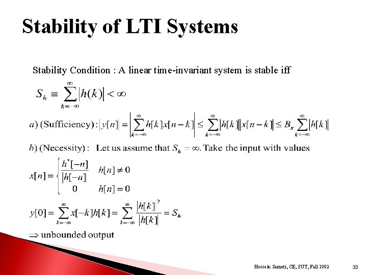
Stability of LTI Systems Stability Condition : A linear time-invariant system is stable iff Hossein Sameti, CE, SUT, Fall 1992 33

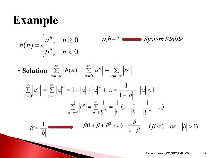
Example a, b=? System Stable • Solution: Hossein Sameti, CE, SUT, Fall 1992 34

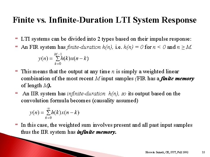
Finite vs. Infinite-Duration LTI System Response LTI systems can be divided into 2 types based on their impulse response: An FIR system has finite-duration h(n), i. e. h(n) = 0 for n < 0 and n ≥ M. This means that the output at any time n is simply a weighted linear combination of the most recent M input samples (FIR has a finite memory of length M). An IIR system has infinite-duration h(n), so its output based on the convolution formula becomes (causality assumed) In this case, the weighted sum involves present and all past input samples thus the IIR system has infinite memory. Hossein Sameti, CE, SUT, Fall 1992 35

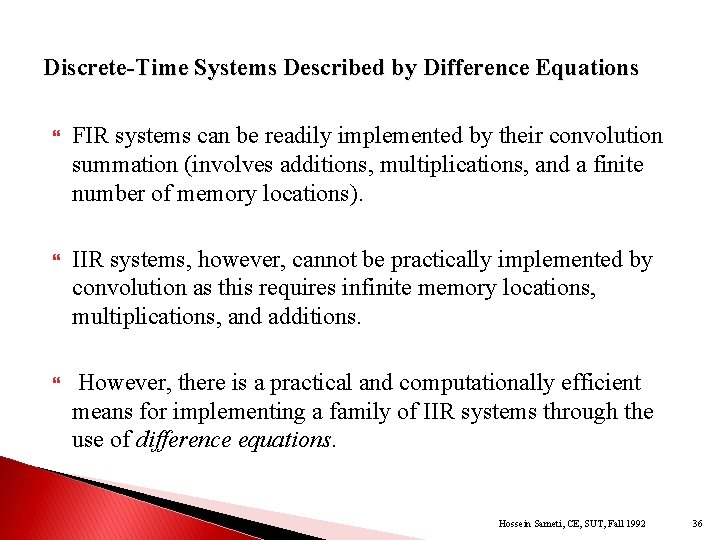
Discrete-Time Systems Described by Difference Equations FIR systems can be readily implemented by their convolution summation (involves additions, multiplications, and a finite number of memory locations). IIR systems, however, cannot be practically implemented by convolution as this requires infinite memory locations, multiplications, and additions. However, there is a practical and computationally efficient means for implementing a family of IIR systems through the use of difference equations. Hossein Sameti, CE, SUT, Fall 1992 36

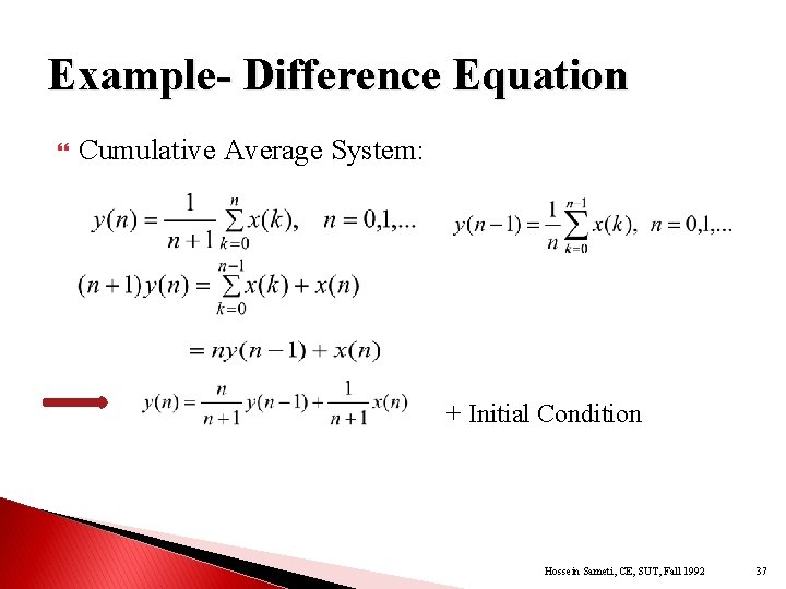
Example- Difference Equation Cumulative Average System: + Initial Condition Hossein Sameti, CE, SUT, Fall 1992 37

Cross-Correlation

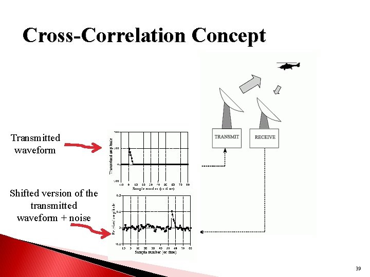
Cross-Correlation Concept Transmitted waveform Shifted version of the transmitted waveform + noise 39

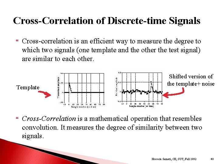
Cross-Correlation of Discrete-time Signals Cross-correlation is an efficient way to measure the degree to which two signals (one template and the other the test signal) are similar to each other. Template Shifted version of the template+ noise Cross-Correlation is a mathematical operation that resembles convolution. It measures the degree of similarity between two signals. Hossein Sameti, CE, SUT, Fall 1992 40

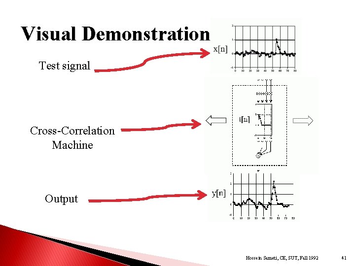
Visual Demonstration Test signal Cross-Correlation Machine Output Hossein Sameti, CE, SUT, Fall 1992 41

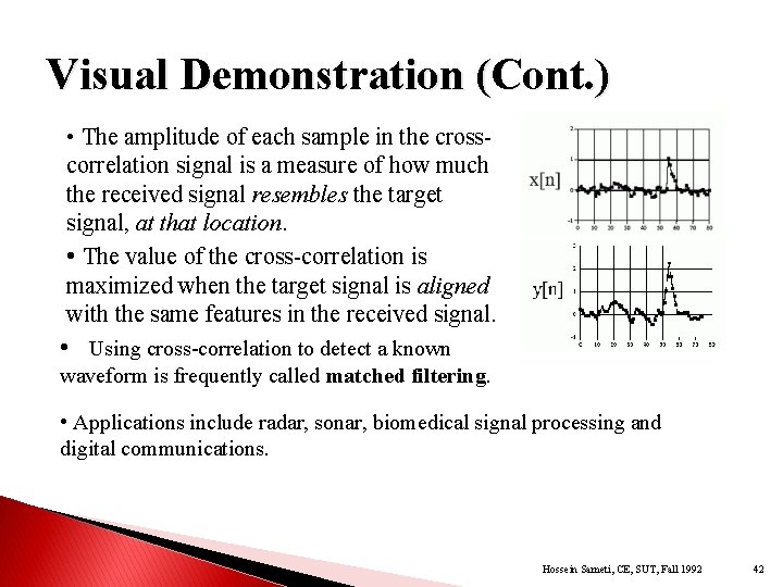
Visual Demonstration (Cont. ) • The amplitude of each sample in the crosscorrelation signal is a measure of how much the received signal resembles the target signal, at that location. • The value of the cross-correlation is maximized when the target signal is aligned with the same features in the received signal. • Using cross-correlation to detect a known waveform is frequently called matched filtering. • Applications include radar, sonar, biomedical signal processing and digital communications. Hossein Sameti, CE, SUT, Fall 1992 42

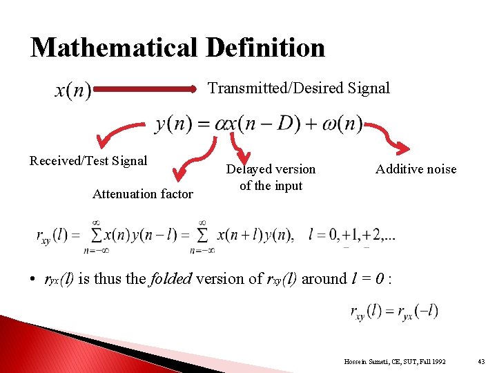
Mathematical Definition Transmitted/Desired Signal Received/Test Signal Attenuation factor Delayed version of the input Additive noise • ryx(l) is thus the folded version of rxy(l) around l = 0 : Hossein Sameti, CE, SUT, Fall 1992 43

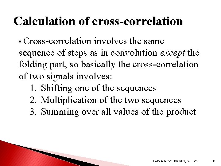
Calculation of cross-correlation • Cross-correlation involves the same sequence of steps as in convolution except the folding part, so basically the cross-correlation of two signals involves: 1. Shifting one of the sequences 2. Multiplication of the two sequences 3. Summing over all values of the product Hossein Sameti, CE, SUT, Fall 1992 44

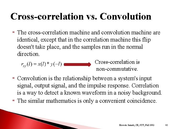
Cross-correlation vs. Convolution The cross-correlation machine and convolution machine are identical, except that in the correlation machine this flip doesn't take place, and the samples run in the normal direction. Cross-correlation is non-commutative. Convolution is the relationship between a system's input signal, output signal, and the impulse response. Correlation is a way to detect a known waveform in a noisy background. The similar mathematics is only a convenient coincidence. Hossein Sameti, CE, SUT, Fall 1992 45

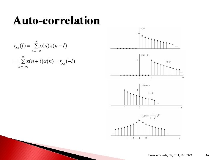
Auto-correlation Hossein Sameti, CE, SUT, Fall 1992 46

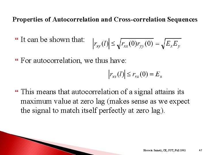
Properties of Autocorrelation and Cross-correlation Sequences It can be shown that: For autocorrelation, we thus have: This means that autocorrelation of a signal attains its maximum value at zero lag (makes sense as we expect the signal to match itself perfectly at zero lag). Hossein Sameti, CE, SUT, Fall 1992 47

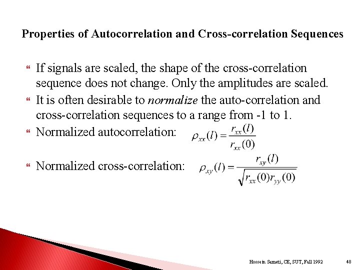
Properties of Autocorrelation and Cross-correlation Sequences If signals are scaled, the shape of the cross-correlation sequence does not change. Only the amplitudes are scaled. It is often desirable to normalize the auto-correlation and cross-correlation sequences to a range from -1 to 1. Normalized autocorrelation: Normalized cross-correlation: Hossein Sameti, CE, SUT, Fall 1992 48

Summary In this lecture, we learned about: Representations of discrete time signals and common basic DT signals Manipulation and representations/diagrams of DT systems Various classification of DT signals: Periodic vs. non-periodic, symmetric vs. anti-symmetric Classifications of DT systems: ◦ Static vs. dynamic, time-invariant vs. time-variant, linear vs. non-linear, causal vs. ◦ non-causal, stable vs. non-stable, FIR vs. IIR LTI systems and their representation Convolution for determining response to arbitrary inputs Cross-correlation Hossein Sameti, CE, SUT, Fall 1992 49