CE 374 K Hydrology Frequency Factors Frequency Analysis

CE 374 K Hydrology Frequency Factors

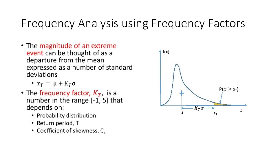
Frequency Analysis using Frequency Factors • f(x) x. T x

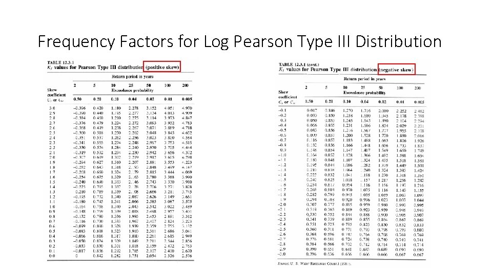
Frequency Factors for Log Pearson Type III Distribution

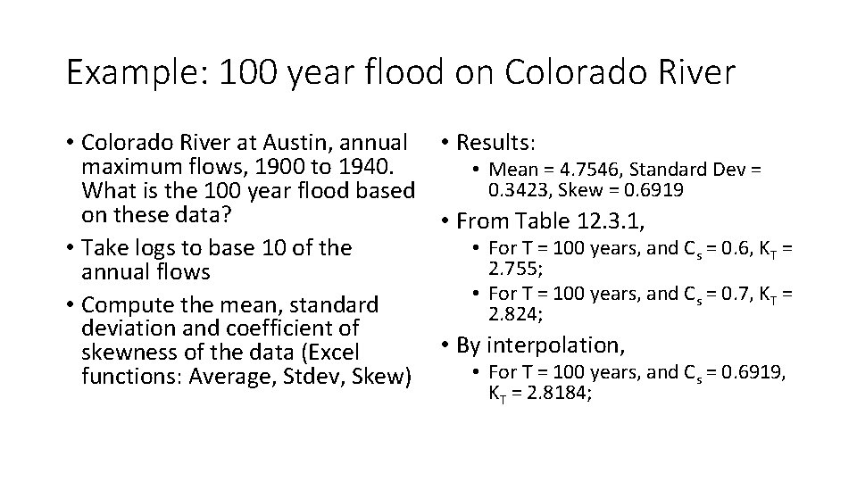
Example: 100 year flood on Colorado River • Colorado River at Austin, annual • Results: maximum flows, 1900 to 1940. • Mean = 4. 7546, Standard Dev = 0. 3423, Skew = 0. 6919 What is the 100 year flood based on these data? • From Table 12. 3. 1, • For T = 100 years, and Cs = 0. 6, KT = • Take logs to base 10 of the 2. 755; annual flows • For T = 100 years, and Cs = 0. 7, KT = • Compute the mean, standard 2. 824; deviation and coefficient of • By interpolation, skewness of the data (Excel • For T = 100 years, and Cs = 0. 6919, functions: Average, Stdev, Skew) KT = 2. 8184;

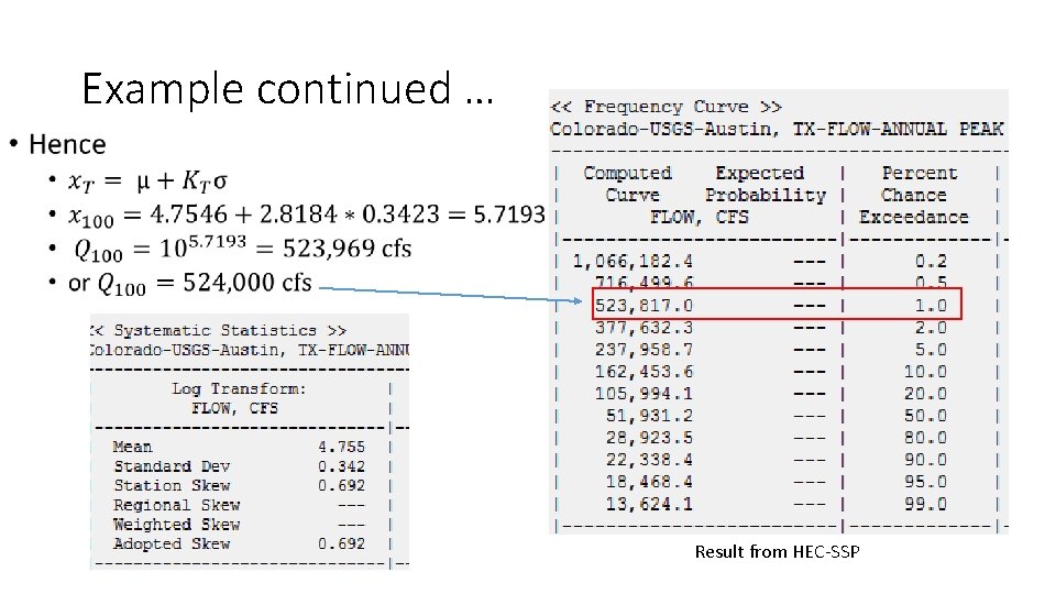
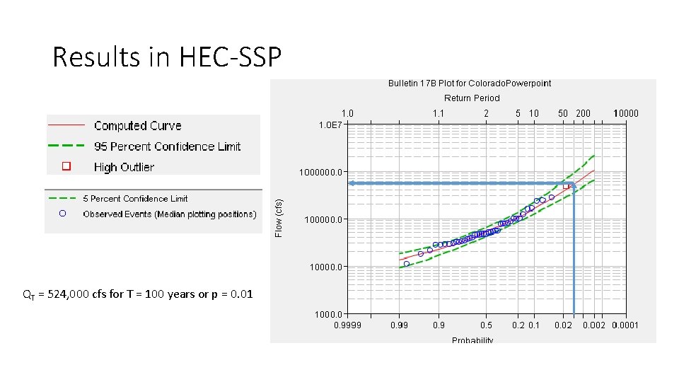
Example continued … • Result from HEC-SSP

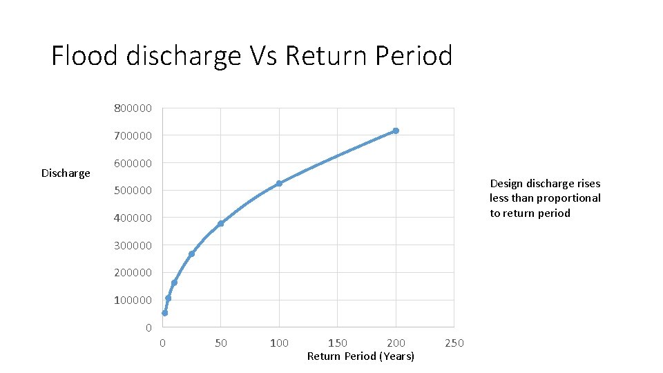
Results in HEC-SSP QT = 524, 000 cfs for T = 100 years or p = 0. 01

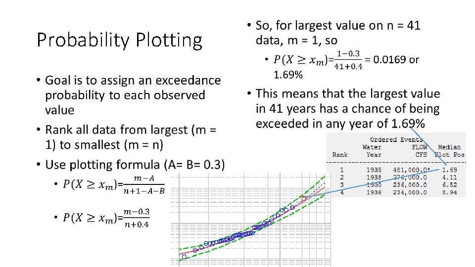
Probability Plotting • •

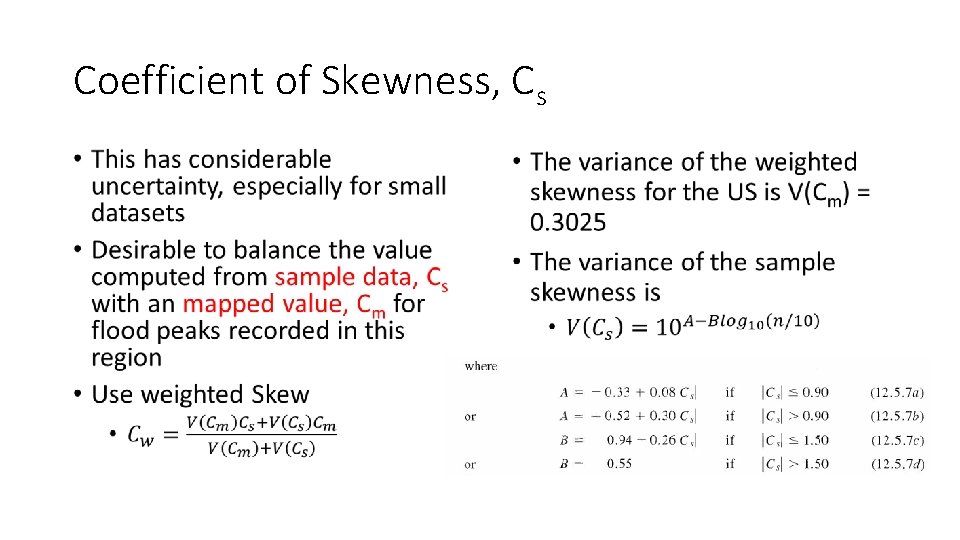
Coefficient of Skewness, Cs • •

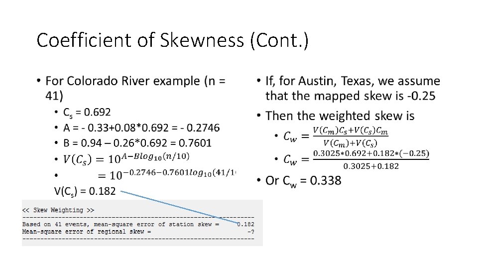
Coefficient of Skewness (Cont. ) • •

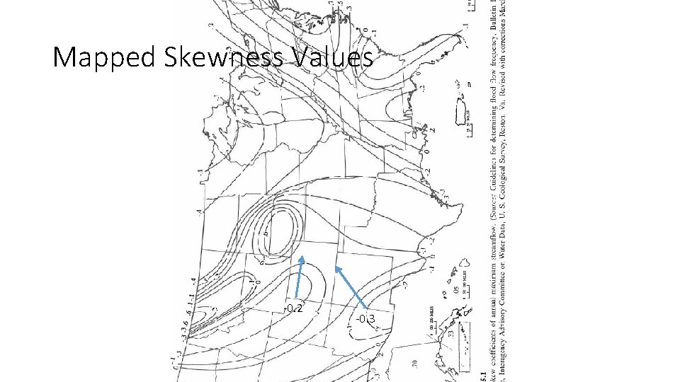
Mapped Skewness Values -0. 2 -0. 3

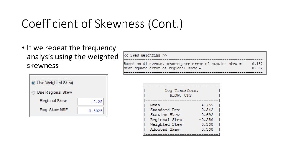
Coefficient of Skewness (Cont. ) • If we repeat the frequency analysis using the weighted skewness

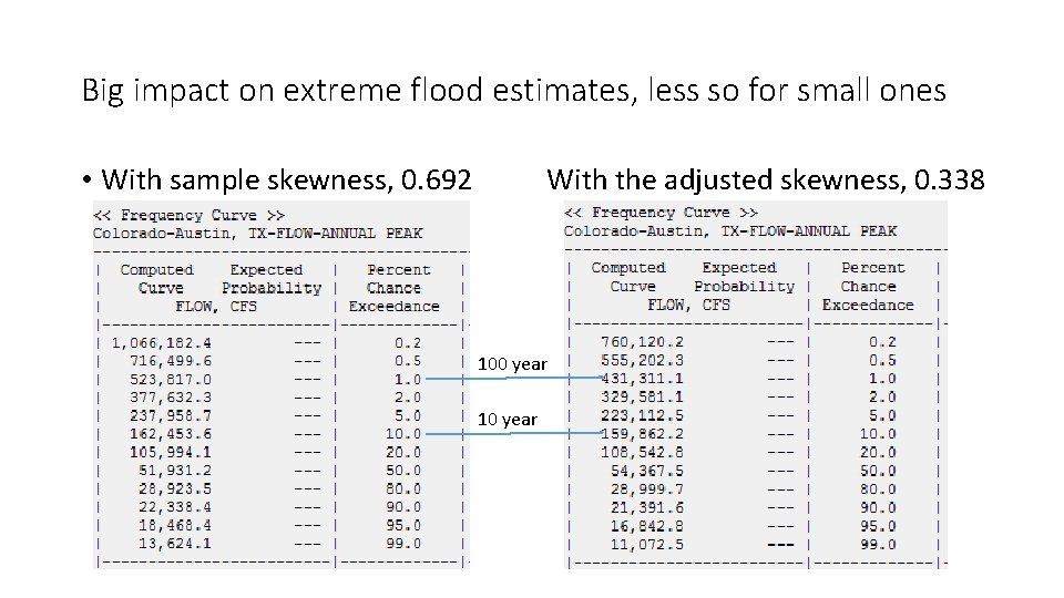
Big impact on extreme flood estimates, less so for small ones • With sample skewness, 0. 692 With the adjusted skewness, 0. 338 100 year 10 year

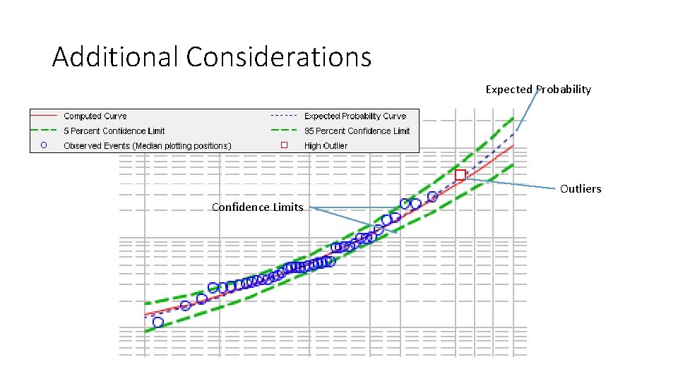
Additional Considerations Expected Probability Outliers Confidence Limits

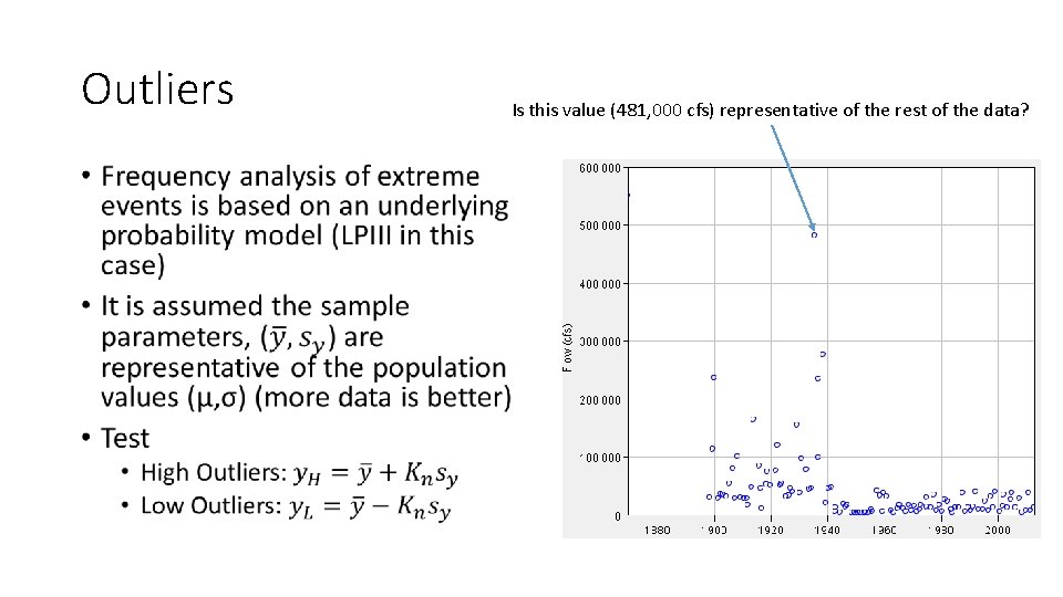
Outliers • Is this value (481, 000 cfs) representative of the rest of the data?

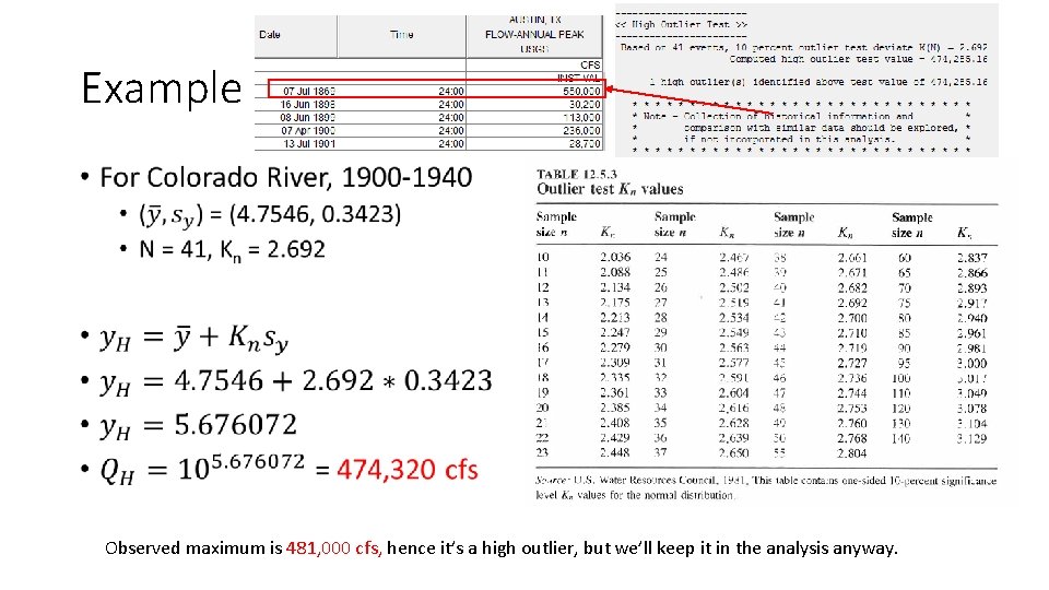
Example • Observed maximum is 481, 000 cfs, hence it’s a high outlier, but we’ll keep it in the analysis anyway.

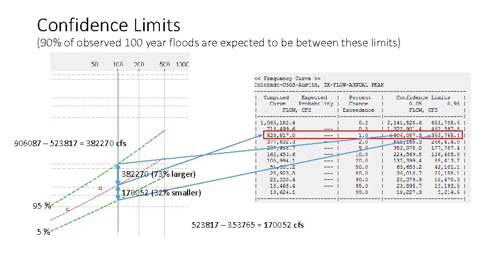
Confidence Limits (90% of observed 100 year floods are expected to be between these limits) 906087 – 523817 = 382270 cfs 382270 (73% larger) 170052 (32% smaller) 95 % 5% 523817 – 353765 = 170052 cfs

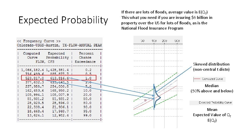
Expected Probability If there are lots of floods, average value is E(QT) This what you need if you are insuring $6 billion in property over the US for lots of floods, as is the National Flood Insurance Program Skewed distribution (non-central t distn) Median (50% above and below) Mean Expected Value of QT E(QT)

Flood discharge Vs Return Period 800000 700000 Discharge 600000 Design discharge rises less than proportional to return period 500000 400000 300000 200000 100000 0 0 50 100 150 200 Return Period (Years) 250