Causality the Basic Framework Imbens and Rubin 2015

Causality: the Basic Framework Imbens and Rubin (2015)

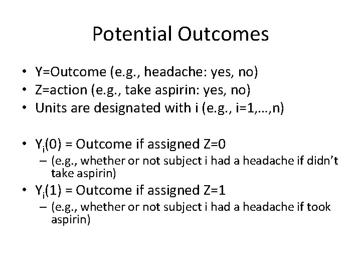
Potential Outcomes • Y=Outcome (e. g. , headache: yes, no) • Z=action (e. g. , take aspirin: yes, no) • Units are designated with i (e. g. , i=1, …, n) • Yi(0) = Outcome if assigned Z=0 – (e. g. , whether or not subject i had a headache if didn’t take aspirin) • Yi(1) = Outcome if assigned Z=1 – (e. g. , whether or not subject i had a headache if took aspirin)

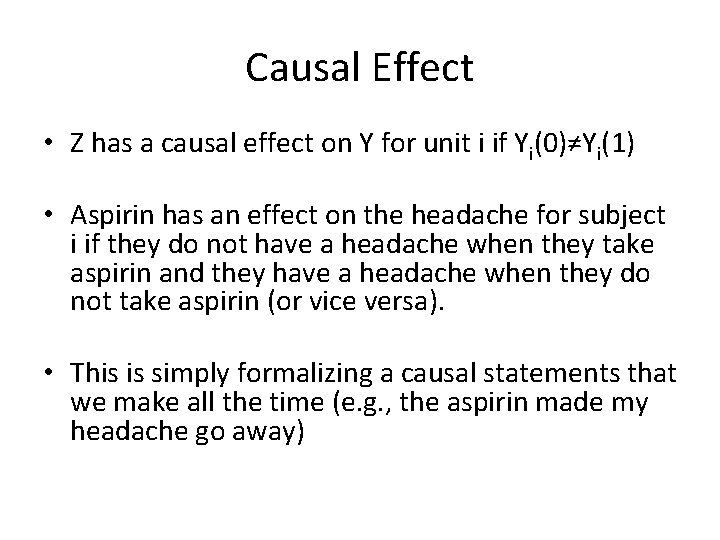
Causal Effect • Z has a causal effect on Y for unit i if Yi(0)≠Yi(1) • Aspirin has an effect on the headache for subject i if they do not have a headache when they take aspirin and they have a headache when they do not take aspirin (or vice versa). • This is simply formalizing a causal statements that we make all the time (e. g. , the aspirin made my headache go away)

Counterfactuals • What would have happened had something different happened. • Many authors treat the terms counterfactuals and potential outcomes synonymously. • Some authors distinguish potential outcomes (the set of possible outcomes, only one of which is realized) from counterfactuals (the set of outcomes that were not realized). • It’s a Wonderful Life

Impossibility of Observing more than one Potential Outcome • Only Yi(0) or Yi(1) can be observed – not both. • Suppose I have a headache on two consecutive days; day 1 I take an aspirin and day 2 I don’t take an aspirin. • Still not observing Yi(0) and Yi(1). • Differences in my surroundings, differences in the severity of the headache, differences in the amount of water I drink with my aspirin – all these things could also affect the outcome and it is impossible to control for all of these things. • This doesn’t mean it’s a bad idea to try (e. g. , crossover trials or making circumstances as constant as possible)

Missing Data Problem • Yiobs=Yi(Zi)=Yi(0) if Zi=0 or Yi(1) if Zi=1. • Yimis=Yi(1 -Zi)=Yi(1) if Zi=0 or Yi(0) if Zi=1. • Causal inference is fundamentally a missing data problem (where at least half of the data are missing).

Average Causal Effects • Consider a set of potential outcomes, {Yi(0), Yi(1)}, for i =1, …, n subjects • [Individual] Causal Effect for subject i – Yi(1)-Yi(0) • Average Causal Effect (ACE): – E[Yi(1)-Yi(0)]=E[Yi(1)]-E[Yi(0)] – Also called Average Treatment Effect (ATE). • Other “average causal effects”: – P[Yi(1)=1]/P[Yi(0)=1] – Median[Yi(1)]-Median[Yi(0)] – Etc.

Standard Assumptions in Rubin Causal Model • SUTVA • Positivity • Random treatment assignment

Stable Unit Treatment Value Assumption (SUTVA) • The potential outcomes for any unit do not vary with the treatments assigned to other units (no interference), and • For each unit, there are no different forms or versions of each treatment level, which lead to different potential outcomes (no hidden variations of treatment). • Rubin (1980)

SUTVA: No interference • Treatment assignment of one unit does not affect the potential outcomes of any other unit. • Probably Realistic: Study of effect of aspirin on headaches. • Probably not Realistic: Study of effect of vaccination on infection in a small population. • No interference allows us to write Yi(Z) instead of Yi(Z), where Z=(Z 1, Z 2, …, Zn). • With binary Z, that means a subject only has 2 potential outcomes instead of 2 n potential outcomes.

SUTVA: No hidden variations of treatment • If Z=aspirin (yes/no), there should be no variations in the type of aspirin (e. g. , some aspirin are stronger than others) • This is basically just an assumption that the treatment is well defined and you know what you’re estimating the causal effect of. • I’ve never been too concerned about this assumption. If there are variations in the treatment, then I would just re-define the treatment to encompass the larger set of treatments (although your knowledge at the end of the study may not be as precise as you’d like) e. g. , pragmatic trials.

Consistency • If Z=z, then Y(z)=Y. • Possible Violation: Intervening on SES (Z) by increasing education has different health consequences (Y) than intervening on SES by increasing income.

Positivity • 0<P(Zi=1)<1 for all i. • This is typically conditional on covariates: • 0<P(Zi=1|Xi)<1 for all i. • You can only measure the causal effect in a population (or subpopulation) if everyone in that population has a non-zero probability of getting either treatment. • Rubin et al. , call this assumption ‘probabilistic assignment’

Random treatment assignment • Yi(0), Yi(1) are independent of Zi for all i. • Treatment assignment is independent of the potential outcomes. • This occurs when treatment is randomly assigned. • Often be made conditional on covariates: – Yi(0), Yi(1) ind. Zi | Xi for all i. • Challenge will be finding covariates in which assumption realistic with observational data. • Other names for approximately the same assumption: – Exchangeability – No unmeasured confounding – Strongly ignorable treatment assignment (actually positivity + random treatment assignment; Rubin et al. )

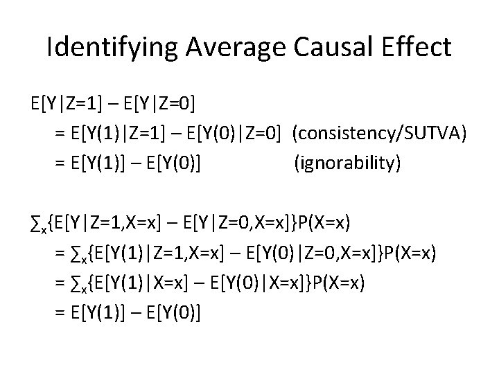
Identifying Average Causal Effect E[Y|Z=1] – E[Y|Z=0] = E[Y(1)|Z=1] – E[Y(0)|Z=0] (consistency/SUTVA) = E[Y(1)] – E[Y(0)] (ignorability) ∑x{E[Y|Z=1, X=x] – E[Y|Z=0, X=x]}P(X=x) = ∑x{E[Y(1)|Z=1, X=x] – E[Y(0)|Z=0, X=x]}P(X=x) = ∑x{E[Y(1)|X=x] – E[Y(0)|X=x]}P(X=x) = E[Y(1)] – E[Y(0)]