Causal Inference Chapter 2 Graphical Models Prof Marco

Causal Inference – Chapter 2 Graphical Models Prof. Marco Zaffalon

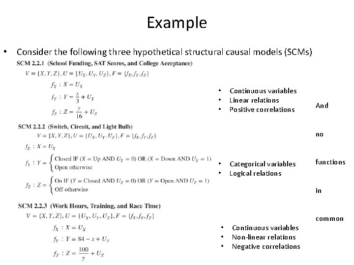
Example • Consider the following three hypothetical structural causal models (SCMs) • • • Continuous variables Linear relations Positive correlations And no • • Categorical variables Logical relations functions in • • • Continuous variables Non-linear relations Negative correlations common

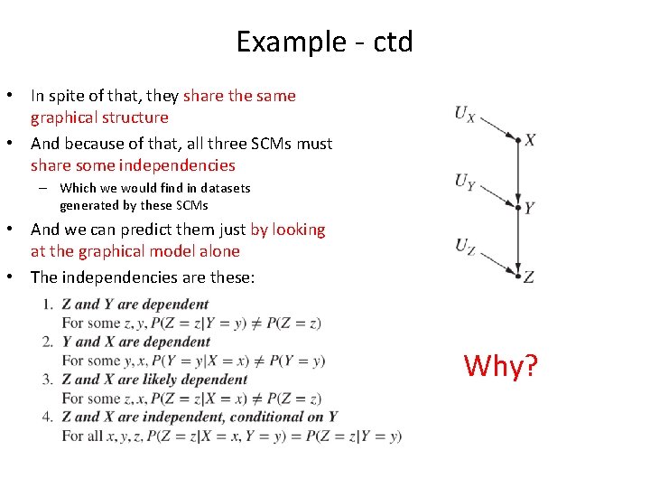
Example - ctd • In spite of that, they share the same graphical structure • And because of that, all three SCMs must share some independencies – Which we would find in datasets generated by these SCMs • And we can predict them just by looking at the graphical model alone • The independencies are these: Why?

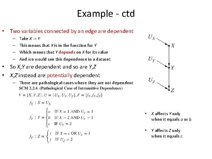
Example - ctd • Two variables connected by an edge are dependent – – Take X -> Y This means that X is in the function for Y Which means that Y depends on X for its value And we would see this dependence in a dataset • So X, Y are dependent and so are Y, Z • X, Z instead are potentially dependent – There are pathological cases where they are not dependent • X affects Y only when it equals a or b • Y affects Z only when it equals c

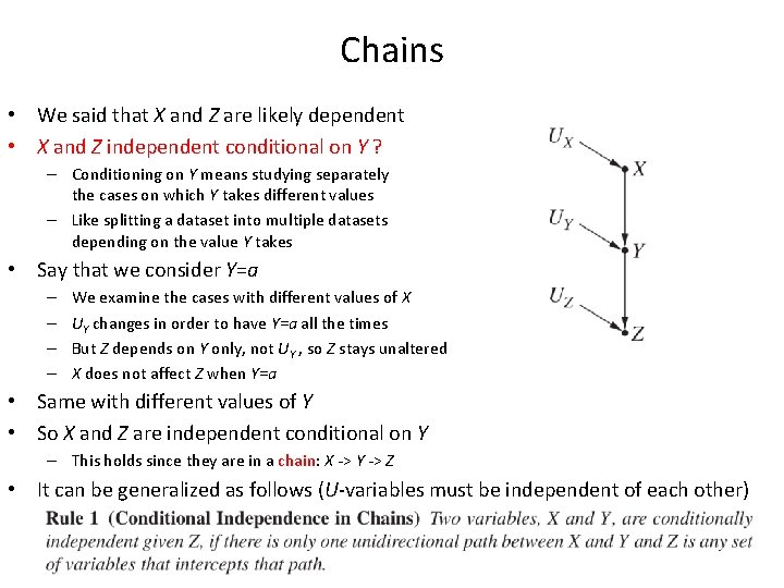
Chains • We said that X and Z are likely dependent • X and Z independent conditional on Y ? – Conditioning on Y means studying separately the cases on which Y takes different values – Like splitting a dataset into multiple datasets depending on the value Y takes • Say that we consider Y=a – – We examine the cases with different values of X UY changes in order to have Y=a all the times But Z depends on Y only, not UY , so Z stays unaltered X does not affect Z when Y=a • Same with different values of Y • So X and Z are independent conditional on Y – This holds since they are in a chain: X -> Y -> Z • It can be generalized as follows (U-variables must be independent of each other)

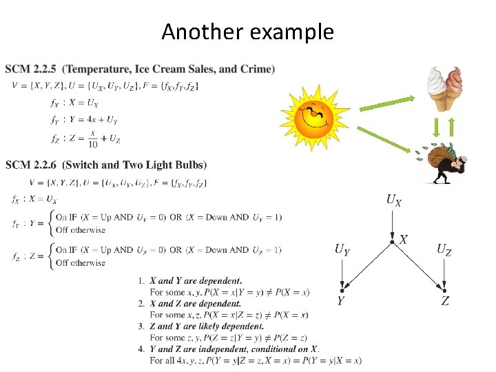
Another example

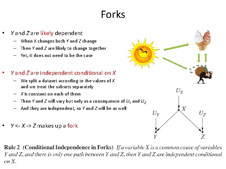
Forks • Y and Z are likely dependent – When X changes both Y and Z change – Then Y and Z are likely to change together – Yet, it does not need to be the case • Y and Z are independent conditional on X – We split a dataset according to the values of X and we treat the subsets separately – X is constant on each of them – Then Y and Z will vary but only as a consequence of UY and UZ – And they are independent, so Y and Z will be as well • Y <- X -> Z makes up a fork

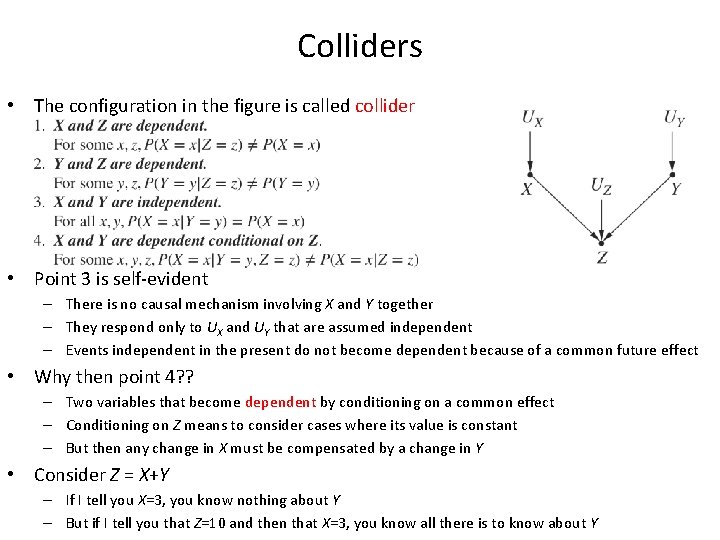
Colliders • The configuration in the figure is called collider • Point 3 is self-evident – There is no causal mechanism involving X and Y together – They respond only to UX and UY that are assumed independent – Events independent in the present do not become dependent because of a common future effect • Why then point 4? ? – Two variables that become dependent by conditioning on a common effect – Conditioning on Z means to consider cases where its value is constant – But then any change in X must be compensated by a change in Y • Consider Z = X+Y – If I tell you X=3, you know nothing about Y – But if I tell you that Z=10 and then that X=3, you know all there is to know about Y

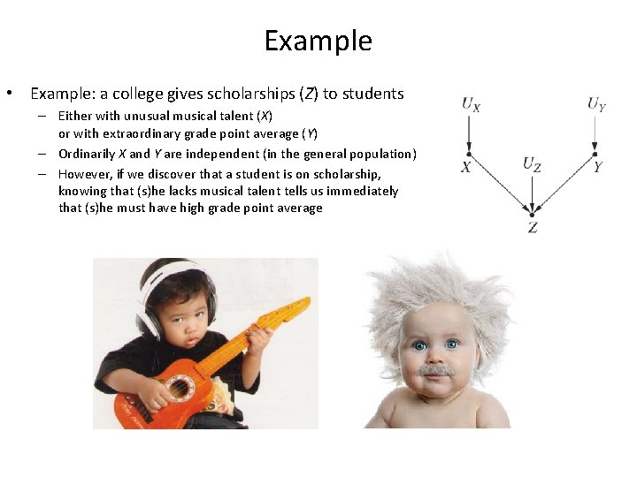
Example • Example: a college gives scholarships (Z) to students – Either with unusual musical talent (X) or with extraordinary grade point average (Y) – Ordinarily X and Y are independent (in the general population) – However, if we discover that a student is on scholarship, knowing that (s)he lacks musical talent tells us immediately that (s)he must have high grade point average

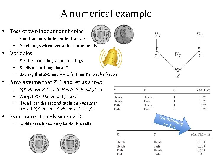
A numerical example • Toss of two independent coins – Simultaneous, independent tosses – A bell rings whenever at least one heads • Variables – X, Y the two coins, Z the bell rings – X tells us nothing about Y – But say that Z=1 and X=Tails, then Y must be heads • Now assume that Z=1 and let us show: – P(X=Heads|Z=1)≠P(X=Heads|Y=Heads, Z=1) – We get P(X=Heads|Z=1) = 2/3 – If we filter the second table on Y=heads: we get P(X=Heads|Y=Heads, Z=1) = 1/2 • Even more strongly when Z=0 – In this case it can only be double tails Cond ition on Z ing =1

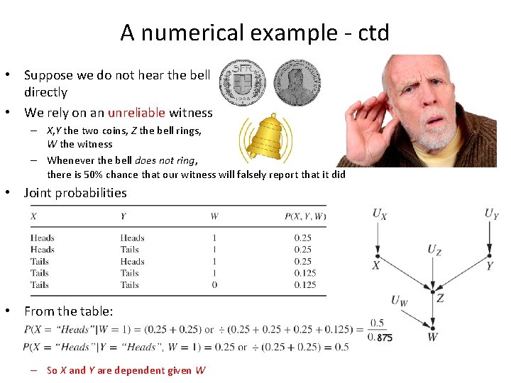
A numerical example - ctd • Suppose we do not hear the bell directly • We rely on an unreliable witness – X, Y the two coins, Z the bell rings, W the witness – Whenever the bell does not ring, there is 50% chance that our witness will falsely report that it did • Joint probabilities • From the table: – So X and Y are dependent given W

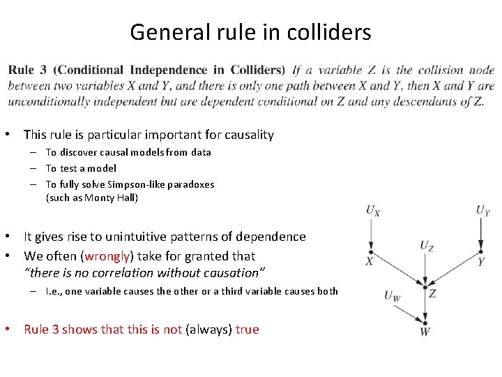
General rule in colliders • This rule is particular important for causality – To discover causal models from data – To test a model – To fully solve Simpson-like paradoxes (such as Monty Hall) • It gives rise to unintuitive patterns of dependence • We often (wrongly) take for granted that “there is no correlation without causation” – I. e. , one variable causes the other or a third variable causes both • Rule 3 shows that this is not (always) true

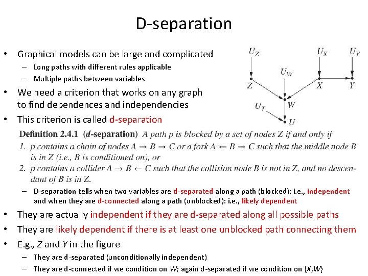
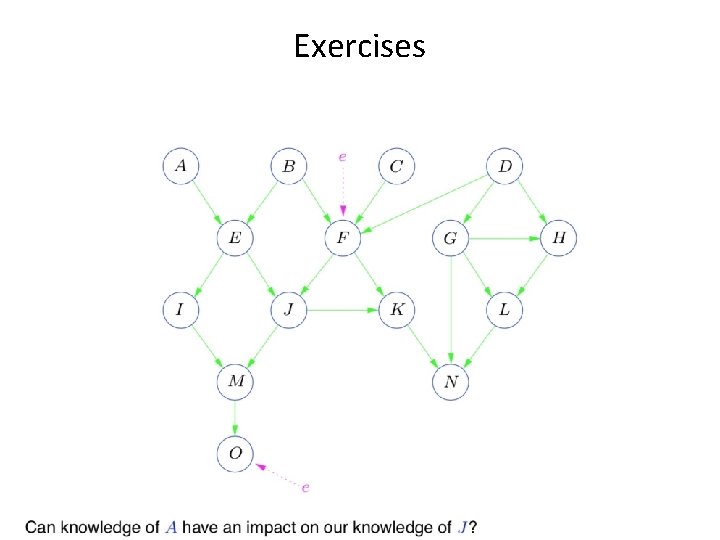
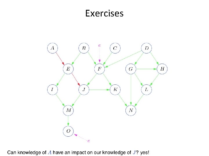
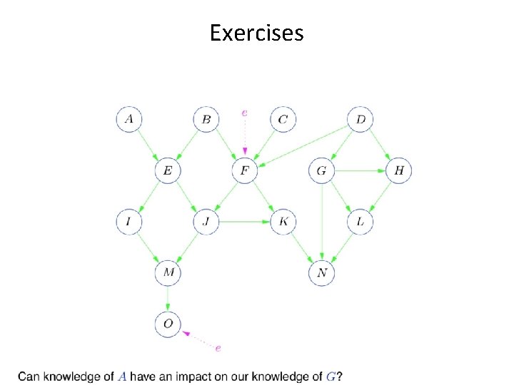
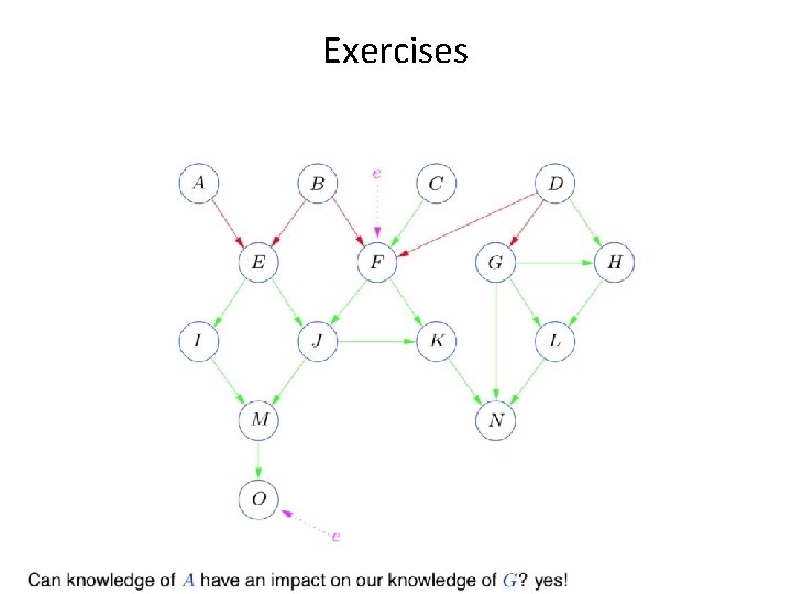
D-separation • Graphical models can be large and complicated – Long paths with different rules applicable – Multiple paths between variables • We need a criterion that works on any graph to find dependences and independencies • This criterion is called d-separation – D-separation tells when two variables are d-separated along a path (blocked): i. e. , independent and when they are d-connected along a path (unblocked): i. e. , likely dependent • They are actually independent if they are d-separated along all possible paths • They are likely dependent if there is at least one unblocked path connecting them • E. g. , Z and Y in the figure – They are d-separated (unconditionally independent) – They are d-connected if we condition on W; again d-separated if we condition on {X, W}

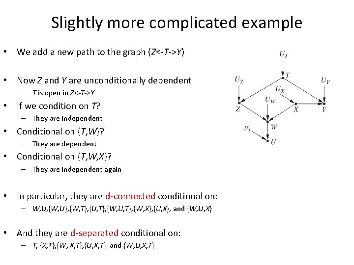
Slightly more complicated example • We add a new path to the graph (Z<-T->Y) • Now Z and Y are unconditionally dependent – T is open in Z<-T->Y • If we condition on T? – They are independent • Conditional on {T, W}? – They are dependent • Conditional on {T, W, X}? – They are independent again • In particular, they are d-connected conditional on: – W, U, {W, U}, {W, T}, {U, T}, {W, X}, {U, X}, and {W, U, X} • And they are d-separated conditional on: – T, {X, T}, {W, X, T}, {U, X, T}, and {W, U, X, T}

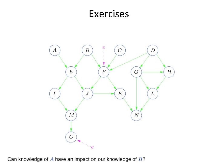
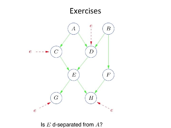
Exercises

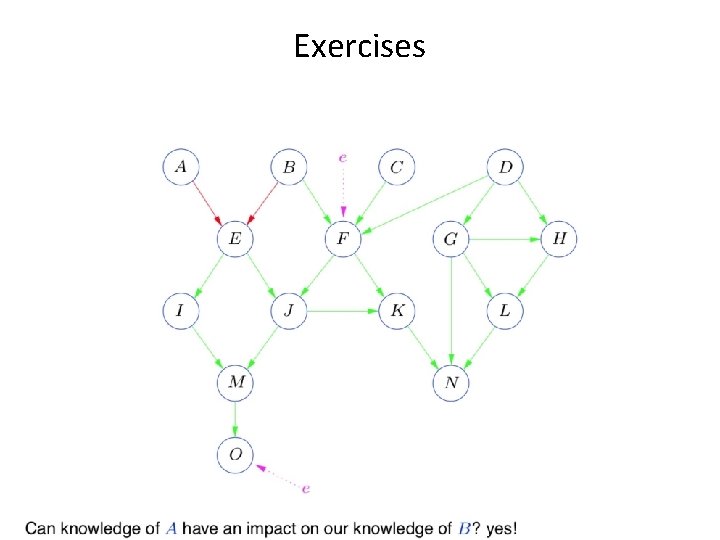
Exercises

Exercises

Exercises

Exercises

Exercises

Exercises

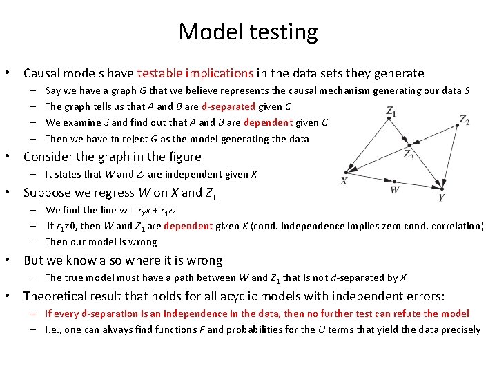
Model testing • Causal models have testable implications in the data sets they generate – – Say we have a graph G that we believe represents the causal mechanism generating our data S The graph tells us that A and B are d-separated given C We examine S and find out that A and B are dependent given C Then we have to reject G as the model generating the data • Consider the graph in the figure – It states that W and Z 1 are independent given X • Suppose we regress W on X and Z 1 – We find the line w = r. Xx + r 1 z 1 – If r 1≠ 0, then W and Z 1 are dependent given X (cond. independence implies zero cond. correlation) – Then our model is wrong • But we know also where it is wrong – The true model must have a path between W and Z 1 that is not d-separated by X • Theoretical result that holds for all acyclic models with independent errors: – If every d-separation is an independence in the data, then no further test can refute the model – I. e. , one can always find functions F and probabilities for the U terms that yield the data precisely

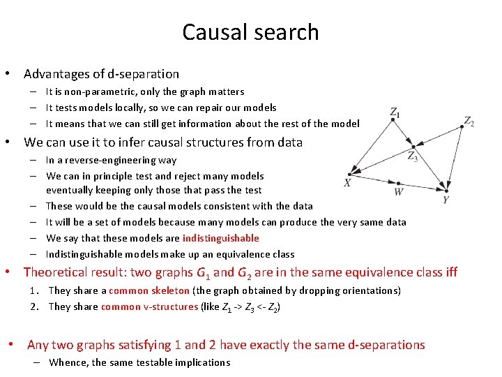
Causal search • Advantages of d-separation – It is non-parametric, only the graph matters – It tests models locally, so we can repair our models – It means that we can still get information about the rest of the model • We can use it to infer causal structures from data – In a reverse-engineering way – We can in principle test and reject many models eventually keeping only those that pass the test – These would be the causal models consistent with the data – It will be a set of models because many models can produce the very same data – We say that these models are indistinguishable – Indistinguishable models make up an equivalence class • Theoretical result: two graphs G 1 and G 2 are in the same equivalence class iff 1. They share a common skeleton (the graph obtained by dropping orientations) 2. They share common v-structures (like Z 1 -> Z 3 <- Z 2) • Any two graphs satisfying 1 and 2 have exactly the same d-separations – Whence, the same testable implications