Causal Effect Estimation with Observational Data Methods and

Causal Effect Estimation with Observational Data: Methods and Applications Part II Michael Lamm and Yiu-Fai Yung SAS Institute 2018 Iowa and Nebraska SAS Users Groups Copyright © SAS Institute Inc. All rights reserved.

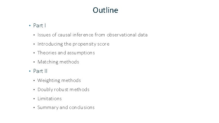
Outline • • Part I • Issues of causal inference from observational data • Introducing the propensity score • Theories and assumptions • Matching methods Part II • Weighting methods • Doubly robust methods • Limitations • Summary and conclusions

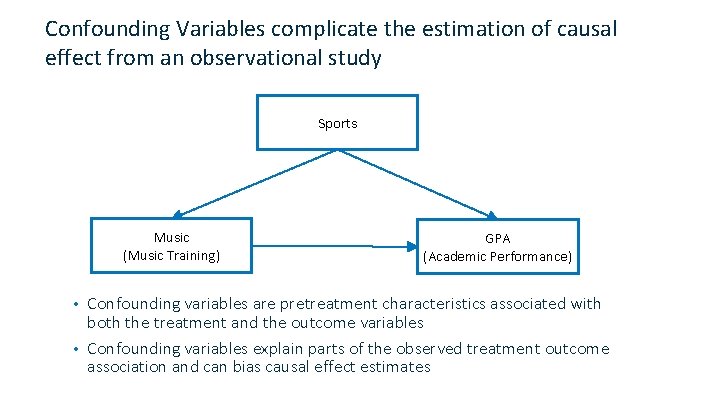
Confounding Variables complicate the estimation of causal effect from an observational study Sports Music (Music Training) GPA (Academic Performance) Confounding variables are pretreatment characteristics associated with both the treatment and the outcome variables • Confounding variables explain parts of the observed treatment outcome association and can bias causal effect estimates •

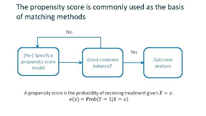
The propensity score is commonly used as the basis of matching methods No (Re-) Specify a propensity score model Yes Good covariate balance? Outcome analysis

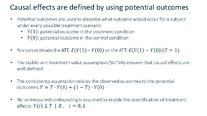
Causal effects are defined by using potential outcomes

Illustration of the Potential Outcomes Framework

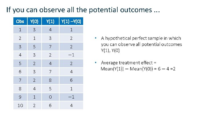
If you can observe all the potential outcomes. . . Obs Y(0) Y(1) –Y(0) 1 3 4 1 2 1 3 2 3 5 7 2 4 3 2 5 2 4 2 6 3 7 4 7 2 8 6 8 4 5 1 9 1 0 10 2 6 4

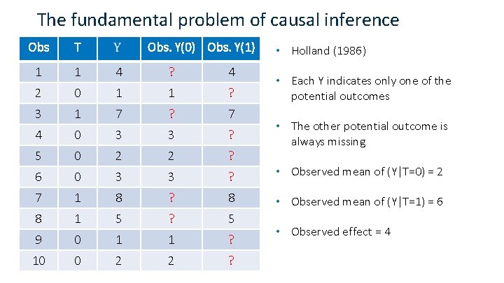
The fundamental problem of causal inference Obs T Obs. Y(0) Obs. Y(1) 1 1 4 ? 4 2 0 1 1 ? 3 1 7 ? 7 4 0 3 3 ? 5 0 2 2 ? 6 0 3 3 ? • Observed mean of (Y|T=0) = 2 7 1 8 ? 8 • Observed mean of (Y|T=1) = 6 8 1 5 ? 5 9 0 1 1 ? 10 0 2 2 ? • Holland (1986) • Each Y indicates only one of the potential outcomes • The other potential outcome is always missing • Observed effect = 4

Propensity Scores Weighting Methods

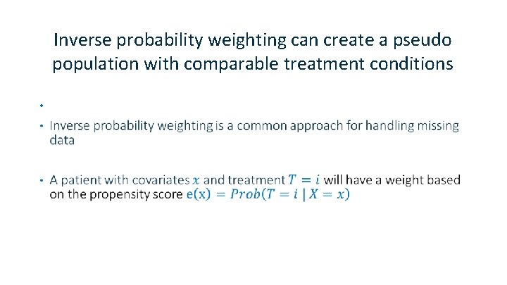
Inverse probability weighting can create a pseudo population with comparable treatment conditions •

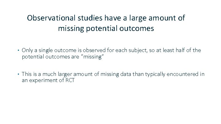
Observational studies have a large amount of missing potential outcomes • Only a single outcome is observed for each subject, so at least half of the potential outcomes are “missing” • This is a much larger amount of missing data than typically encountered in an experiment of RCT

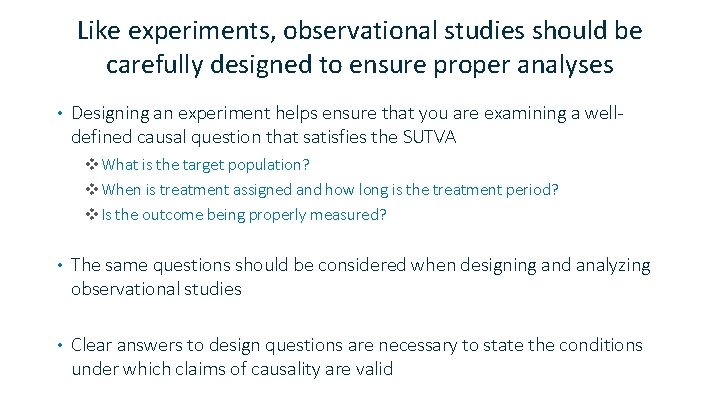
Like experiments, observational studies should be carefully designed to ensure proper analyses • Designing an experiment helps ensure that you are examining a welldefined causal question that satisfies the SUTVA v. What is the target population? v. When is treatment assigned and how long is the treatment period? v. Is the outcome being properly measured? • The same questions should be considered when designing and analyzing observational studies • Clear answers to design questions are necessary to state the conditions under which claims of causality are valid

Example 3. Propensity Scores Weighting Methods

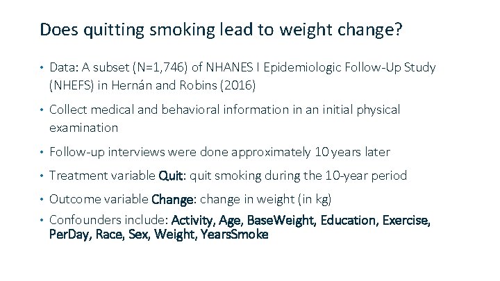
Does quitting smoking lead to weight change? • Data: A subset (N=1, 746) of NHANES I Epidemiologic Follow-Up Study (NHEFS) in Hernán and Robins (2016) • Collect medical and behavioral information in an initial physical examination • Follow-up interviews were done approximately 10 years later • Treatment variable Quit: quit smoking during the 10 -year period Outcome variable Change: change in weight (in kg) • Confounders include: Activity, Age, Base. Weight, Education, Exercise, Per. Day, Race, Sex, Weight, Years. Smoke •

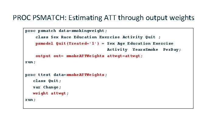
PROC PSMATCH: Estimating ATT through output weights proc psmatch data=smokingweight; class Sex Race Education Exercise Activity Quit ; psmodel Quit(Treated='1') = Sex Age Education Exercise Activity Years. Smoke Per. Day; output out= smoke. ATTWeights attwgt=attwgt; run; proc ttest data=smoke. ATTWeights; class Quit; var Change; weight attwgt; run;

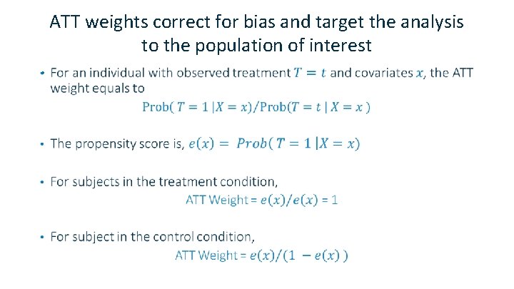
ATT weights correct for bias and target the analysis to the population of interest •

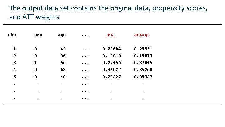
The output data set contains the original data, propensity scores, and ATT weights Obs sex age . . . _PS_ attwgt 1 0 42 . . . 0. 20604 0. 25951 2 0 36 . . . 0. 16018 0. 19073 3 1 56 . . . 0. 27455 0. 37845 4 0 68 . . . 0. 46022 0. 85260 5 0 40 . . . 0. 28227 0. 39327 . . .

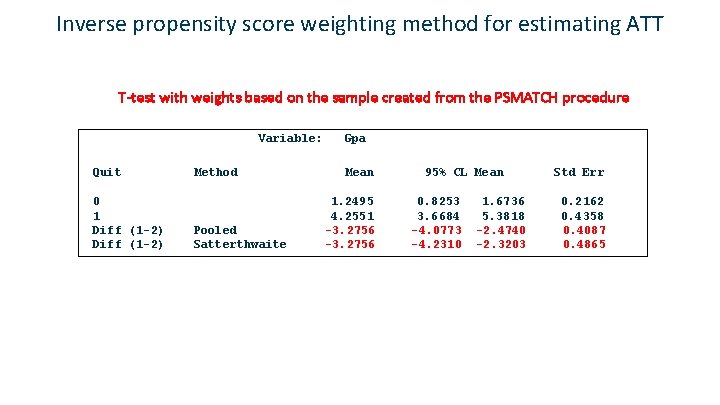
Inverse propensity score weighting method for estimating ATT T-test with weights based on the sample created from the PSMATCH procedure Variable: Quit 0 1 Diff (1 -2) Method Pooled Satterthwaite Gpa Mean 1. 2495 4. 2551 -3. 2756 95% CL Mean 0. 8253 3. 6684 -4. 0773 -4. 2310 1. 6736 5. 3818 -2. 4740 -2. 3203 Std Err 0. 2162 0. 4358 0. 4087 0. 4865

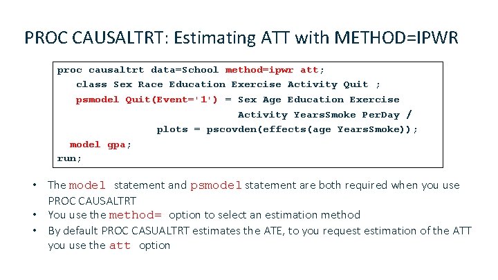
PROC CAUSALTRT: Estimating ATT with METHOD=IPWR proc causaltrt data=School method=ipwr att; class Sex Race Education Exercise Activity Quit ; psmodel Quit(Event='1') = Sex Age Education Exercise Activity Years. Smoke Per. Day / plots = pscovden(effects(age Years. Smoke)); model gpa; run; • The model statement and psmodel statement are both required when you use PROC CAUSALTRT • You use the method= option to select an estimation method • By default PROC CASUALTRT estimates the ATE, to you request estimation of the ATT you use the att option

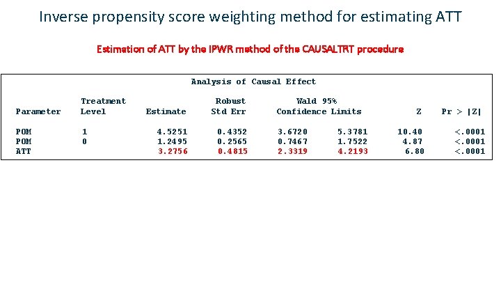
Inverse propensity score weighting method for estimating ATT Estimation of ATT by the IPWR method of the CAUSALTRT procedure Analysis of Causal Effect Parameter POM ATT Treatment Level 1 0 Estimate Robust Std Err 4. 5251 1. 2495 3. 2756 0. 4352 0. 2565 0. 4815 Wald 95% Confidence Limits 3. 6720 0. 7467 2. 3319 5. 3781 1. 7522 4. 2193 Z 10. 40 4. 87 6. 80 Pr > |Z| <. 0001

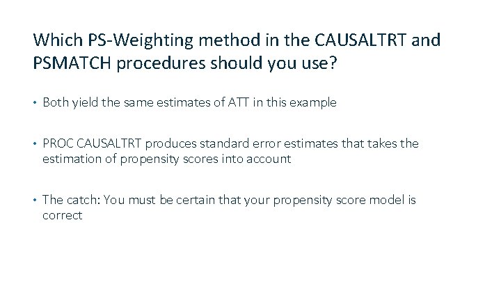
Which PS-Weighting method in the CAUSALTRT and PSMATCH procedures should you use? • Both yield the same estimates of ATT in this example • PROC CAUSALTRT produces standard error estimates that takes the estimation of propensity scores into account • The catch: You must be certain that your propensity score model is correct

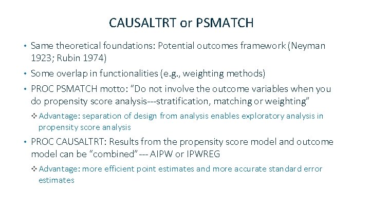
CAUSALTRT or PSMATCH Same theoretical foundations: Potential outcomes framework (Neyman 1923; Rubin 1974) • Some overlap in functionalities (e. g. , weighting methods) • PROC PSMATCH motto: “Do not involve the outcome variables when you do propensity score analysis---stratification, matching or weighting” • v Advantage: separation of design from analysis enables exploratory analysis in propensity score analysis • PROC CAUSALTRT: Results from the propensity score model and outcome model can be “combined”--- AIPW or IPWREG v Advantage: more efficient point estimates and more accurate standard error estimates

Regression Adjustment and Doubly Robust Methods

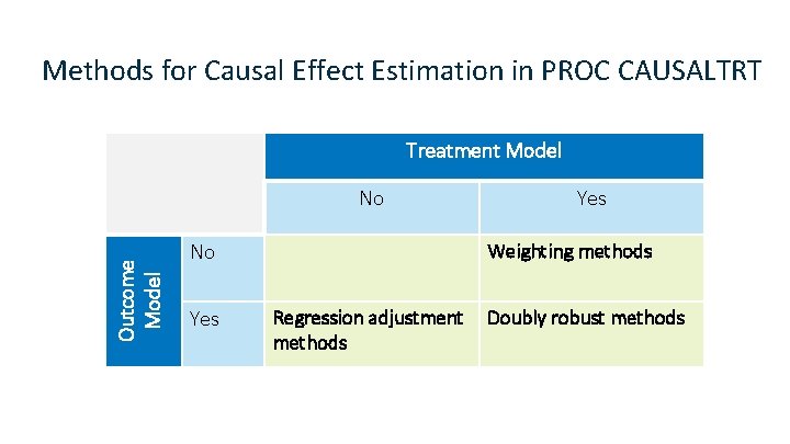
Methods for Causal Effect Estimation in PROC CAUSALTRT Treatment Model Outcome Model No No Yes Weighting methods Regression adjustment methods Doubly robust methods

Regression Adjustment Method • Estimation by regression adjustment performs the following steps: Fit models for the outcome separately within each of the treatment conditions • Compute predicted outcomes for each subject from these models • Use the predicted values to estimate the treatment effect of interest • • METHOD=REGADJ option in PROC CAUSALTRT

Considerations when using regression adjustment • The method is dependent on a correctly specified outcome model v. Incorrectly specified outcome models can lead to biased model estimates and biased treatment effects • Extrapolation might be a concern if covariate distributions in treatment conditions are systematically different

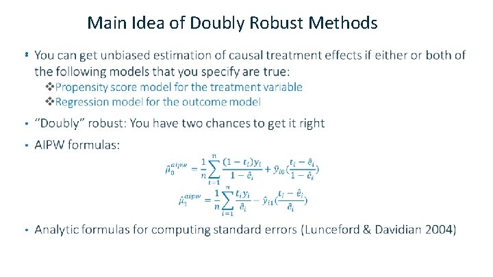
Doubly Robust Methods of PROC CAUSALTRT • Augmented inverse probability weighting v Estimate the propensity score and perform weighing v Augment weighting by using predicted outcome values v METHOD=AIPW in PROC CAUSALTRT • Inverse probability weighted regression v Estimate the propensity scores v Fit outcome models with inverse probability weights v Estimate the causal effects by using predicted values from v METHOD=IPWREG in PROC CAUSALTRT

Main Idea of Doubly Robust Methods •

Example 4. AIPW Example

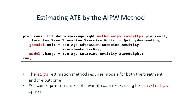
Estimating ATE by the AIPW Method proc causaltrt data=smokingweight method=aipw covdiffps plots=all; class Sex Race Education Exercise Activity Quit /descending; psmodel Quit = Sex Age Education Exercise Activity Years. Smoke Per. Day; model Change = Sex Age Exercise Activity Base. Weight; run; • The aipw estimation method requires models for both the treatment and the outcome • You can request measures of covariate balance by using the covdiffps option

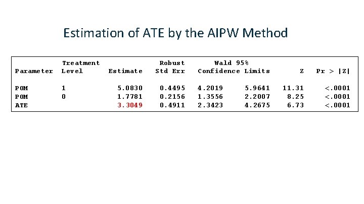
Estimation of ATE by the AIPW Method Parameter POM ATE Treatment Level 1 0 Estimate Robust Std Err 5. 0830 1. 7781 3. 3049 0. 4495 0. 2156 0. 4911 Wald 95% Confidence Limits 4. 2019 1. 3556 2. 3423 5. 9641 2. 2007 4. 2675 Z Pr > |Z| 11. 31 8. 25 6. 73 <. 0001

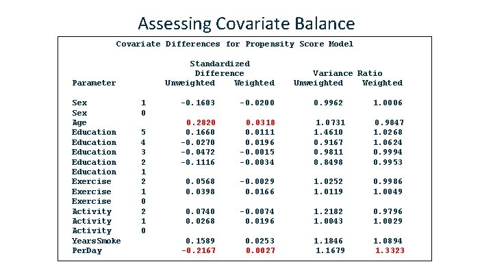
Assessing Covariate Balance Covariate Differences for Propensity Score Model Standardized Difference Unweighted Weighted Parameter Sex Age Education Education Exercise Activity Years. Smoke Per. Day 1 0 5 4 3 2 1 0 Variance Ratio Unweighted Weighted -0. 1603 -0. 0200 0. 9962 1. 0006 0. 2820 0. 1660 -0. 0270 -0. 0472 -0. 1116 0. 0318 0. 0111 0. 0196 -0. 0015 -0. 0034 1. 0731 1. 4610 0. 9167 0. 9811 0. 8498 0. 9847 1. 0268 1. 0624 0. 9994 0. 9953 0. 0568 0. 0398 -0. 0029 0. 0166 1. 0252 1. 0119 0. 9986 1. 0049 0. 0740 0. 0268 -0. 0074 0. 0196 1. 2182 1. 0043 0. 9796 1. 0029 0. 1589 -0. 2167 0. 0253 0. 0027 1. 1846 1. 1679 1. 0894 1. 3323

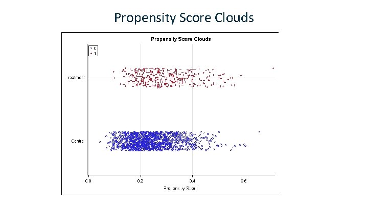
Propensity Score Clouds

Example 4. Limitations

Family Aid and Child Development • A subset of data from the 1997 Child Development Supplement to the Panel Study of Income Dynamics (Hofferth et al. 2001; Guo and Fraser 2015) • Treatment variable AFDC: Receiving welfare benefit • Outcome variables Lwi: child’s development, as measured by the agenormalized letter-word identification portion of the Woodcock-Johnson Tests for Achievement • N=1, 003 children whose primary caregiver was less than 36 years old

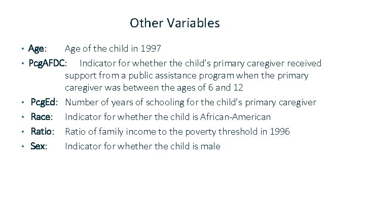
Other Variables • • • Age: Age of the child in 1997 Pcg. AFDC: Indicator for whether the child’s primary caregiver received support from a public assistance program when the primary caregiver was between the ages of 6 and 12 Pcg. Ed: Number of years of schooling for the child’s primary caregiver Race: Indicator for whether the child is African-American Ratio: Ratio of family income to the poverty threshold in 1996 Sex: Indicator for whether the child is male

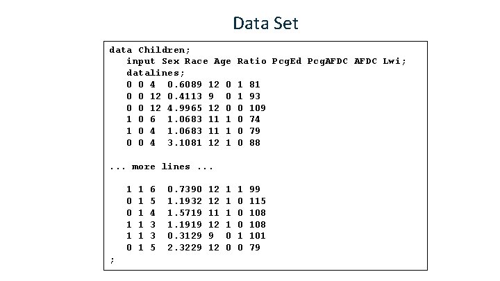
Data Set data Children; input Sex Race Age datalines; 0 0 4 0. 6089 12 0 0 0 12 0. 4113 9 0 0 0 12 4. 9965 12 0 1 0 6 1. 0683 11 1 1 0 4 1. 0683 11 1 0 0 4 3. 1081 12 1 Ratio Pcg. Ed Pcg. AFDC Lwi; 1 1 0 0 81 93 109 74 79 88 1 0 0 0 1 0 99 115 108 101 79 . . . more lines. . . 1 0 0 1 1 0 ; 1 1 1 6 5 4 3 3 5 0. 7390 1. 1932 1. 5719 1. 1919 0. 3129 2. 3229 12 12 11 12 9 12 1 1 0 0

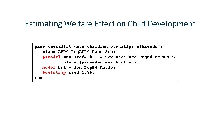
Estimating Welfare Effect on Child Development proc causaltrt data=Children covdiffps nthreads=2; class AFDC Pcg. AFDC Race Sex; psmodel AFDC(ref='0') = Sex Race Age Pcg. Ed Pcg. AFDC/ plots=(pscovden weightcloud); model Lwi = Sex Pcg. Ed Ratio; bootstrap seed=1776; run;

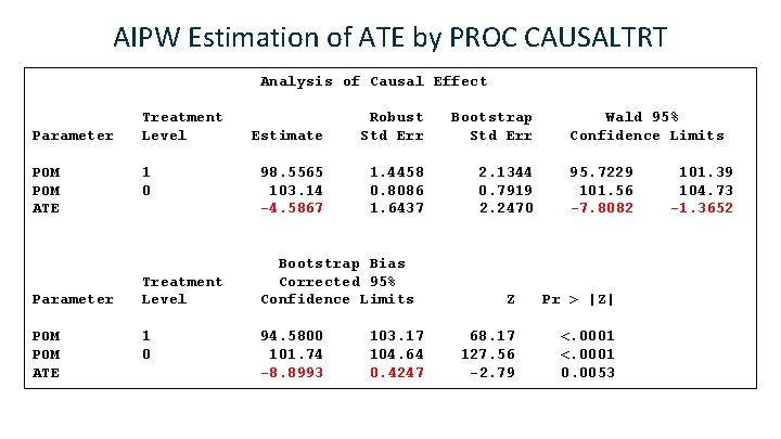
AIPW Estimation of ATE by PROC CAUSALTRT Analysis of Causal Effect Parameter POM POM ATE Treatment Level 1 0 Estimate Robust Std Err Bootstrap Std Err 98. 5565 103. 14 -4. 5867 1. 4458 0. 8086 1. 6437 2. 1344 0. 7919 2. 2470 Bootstrap Bias Corrected 95% Confidence Limits 94. 5800 101. 74 -8. 8993 103. 17 104. 64 0. 4247 Wald 95% Confidence Limits 95. 7229 101. 56 -7. 8082 Z Pr > |Z| 68. 17 127. 56 -2. 79 <. 0001 0. 0053 101. 39 104. 73 -1. 3652

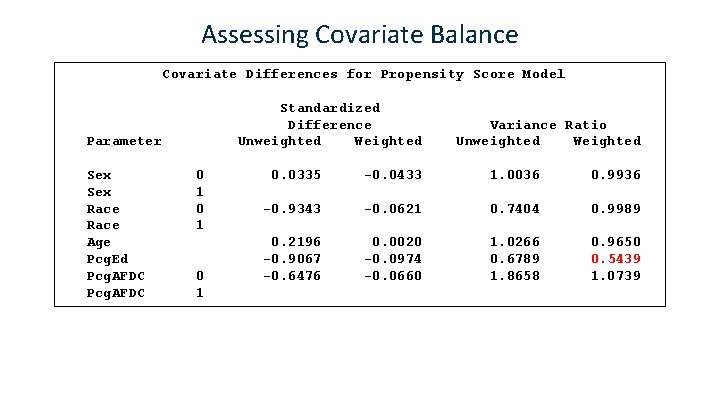
Assessing Covariate Balance Covariate Differences for Propensity Score Model Standardized Difference Unweighted Weighted Parameter Sex Race Age Pcg. Ed Pcg. AFDC 0 1 0 1 Variance Ratio Unweighted Weighted 0. 0335 -0. 0433 1. 0036 0. 9936 -0. 9343 -0. 0621 0. 7404 0. 9989 0. 2196 -0. 9067 -0. 6476 0. 0020 -0. 0974 -0. 0660 1. 0266 0. 6789 1. 8658 0. 9650 0. 5439 1. 0739

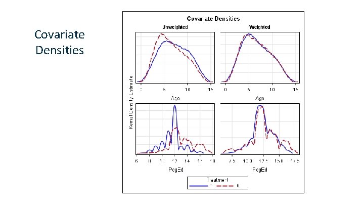
Covariate Densities

Other Types of Propensity Score Models • PROC PSMATCH uses logistic regression models for estimating propensity scores • If a propensity score model does not lead to good covariate balance, what can you do? v Use another set of predictors in the logistic model v Use another type of model

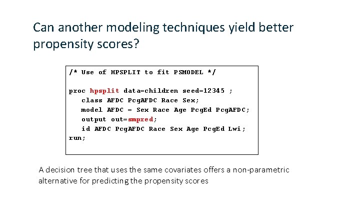
Can another modeling techniques yield better propensity scores? /* Use of HPSPLIT to fit PSMODEL */ proc hpsplit data=children seed=12345 ; class AFDC Pcg. AFDC Race Sex; model AFDC = Sex Race Age Pcg. Ed Pcg. AFDC; output out=smpred; id AFDC Pcg. AFDC Race Sex Age Pcg. Ed Lwi; run; A decision tree that uses the same covariates offers a non-parametric alternative for predicting the propensity scores

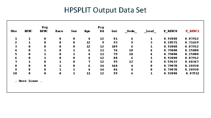
HPSPLIT Output Data Set Obs AFDC 1 2 3 4 5 6 7 8 9 10 1 1 0 0 0 Pcg AFDC … More lines … 0 0 0 1 1 1 0 0 Race 0 0 0 1 1 1 0 Sex 0 0 0 1 1 Age Pcg Ed Lwi _Node_ 4 12 12 6 4 4 7 6 4 11 12 9 12 11 11 12 12 14 14 12 81 93 109 74 79 88 95 140 84 99 6 10 10 6 12 4 4 6 _Leaf_ 1 3 1 4 4 1 6 0 0 1 P_AFDC 0 P_AFDC 1 0. 92088 0. 28571 0. 92088 0. 75000 0. 92088 0. 59633 0. 79070 0. 92088 0. 07912 0. 71429 0. 07912 0. 25000 0. 07912 0. 40367 0. 20930 0. 07912

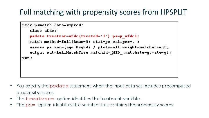
Full matching with propensity scores from HPSPLIT proc psmatch data=smpred; class afdc; psdata treatvar=afdc(treated='1') ps=p_afdc 1; match method=full(kmax=5) stat=ps caliper=. ; assess ps var=(age Pcg. Ed) / plots=all weight=matchatewgt; output out=full. Match. Tree matchid=_MID_ matchatewgt=atewgt; run; • You specify the psdata statement when the input data set includes precomputed propensity scores • The treatvar= option identifies the treatment variable • The ps= option identifies the variable that contains the propensity scores

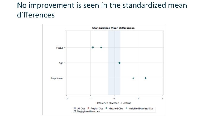
No improvement is seen in the standardized mean differences

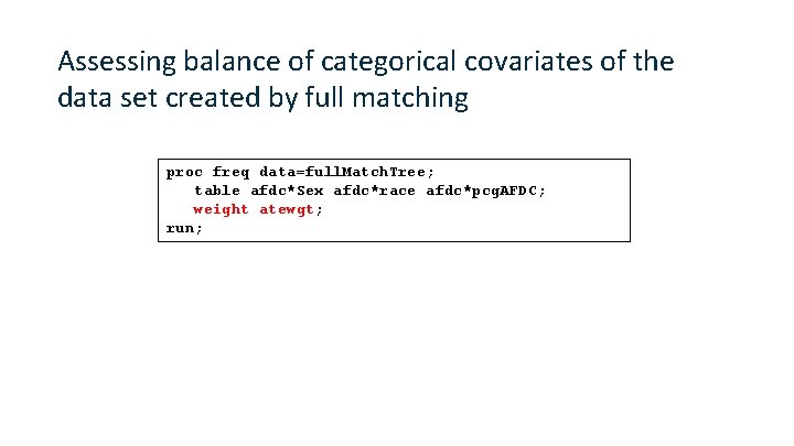
Assessing balance of categorical covariates of the data set created by full matching proc freq data=full. Match. Tree; table afdc*Sex afdc*race afdc*pcg. AFDC; weight atewgt; run;

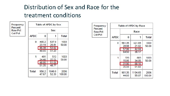
Distribution of Sex and Race for the treatment conditions

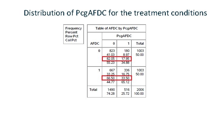
Distribution of Pcg. AFDC for the treatment conditions

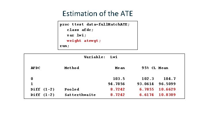
Estimation of the ATE proc ttest data=full. Match. ATE; class afdc; var lwi; weight atewgt; run; Variable: AFDC 0 1 Diff (1 -2) Method Pooled Satterthwaite Lwi Mean 103. 5 94. 7856 8. 7242 95% CL Mean 102. 3 93. 0614 6. 7855 6. 6174 104. 7 96. 5099 10. 6629 10. 8309

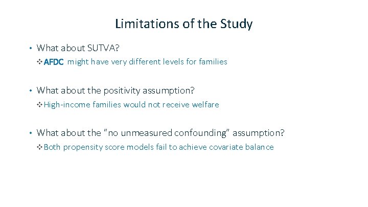
Limitations of the Study • What about SUTVA? v AFDC might have very different levels for families • What about the positivity assumption? v High-income families would not receive welfare • What about the “no unmeasured confounding” assumption? v Both propensity score models fail to achieve covariate balance

Summary of causal effect estimation • Confounding in observational studies must be dealt with • Under the potential outcomes framework, causal interpretations of the effects are possible if assumptions are satisfied • You can use various methods for estimating average treatment effect (ATE) and average treatment effect for the treated (ATT) • Assessing covariate balance is important

Introductory Books and Articles • Austin, P. C. (2011). “An Introduction to Propensity Score Methods for Reducing the Effects of Confounding in Observational Studies. ” Multivariate Behavioral Research 46: 399– 424. • Hernán and Robins (2016). Causal Inference. Boca Raton, FL: Chapman & Hall/CRC. Forthcoming. • Guo, S. , and Fraser, M. W. (2015). Propensity Score Analysis: Statistical Methods and Applications (2 nd ed. ). Thousand Oaks, CA: Sage Publications. • Morgan, S. L. , and Winship, C. (2015). Counterfactuals and Causal Inference: Methods and Principles for Social Research (2 nd ed. ). New York: Cambridge University Press. • Pan, W. , and Bai, H (2015). Propensity Score Analysis: Fundamentals and Developments. New York: The Guilford Press. • Stuart, E. A. (2010). “Matching Methods for Causal Inference: A Review and a Look Forward. ” Statistical Science 25: 1– 21. SAS Global Forum Papers • • • Lamm, M. , and Yung, Y. F. (2017). “Estimating Causal Effects from Observational Data with the CAUSALTRT procedure. ” In Proceedings of the SAS Global Forum 2017 Conference. Cary, NC: SAS Institute Inc. http: //support. sas. com/resources/papers/proceedings 17/SAS 0374 -2017. pdf Yang, Y. , Yung, Y. F. , and Stokes, M. (2017). “Propensity Score Methods for Causal Inference with the PSMATCH Procedure. ” In Proceedings of the SAS Global Forum 2017 Conference. Cary, NC: SAS Institute Inc. http: //support. sas. com/resources/papers/proceedings 17/SAS 0332 -2017. pdf Yung, Y. F. , Lamm. M, and Zhang. W (2018). “Causal Mediation Analysis with the CAUSALMED Procedure. ” In Proceedings of the SAS Global Forum 2017 Conference. Cary, NC: SAS Institute Inc.