Causal Effect Estimation with Observational Data Methods and

Causal Effect Estimation with Observational Data: Methods and Applications Part I Michael Lamm and Yiu-Fai Yung SAS Institute 2018 Iowa and Nebraska SAS Users Groups Copyright © SAS Institute Inc. All rights reserved.

The central issue is about how to … … estimate causal effects from observational data.

Causal analysis can address some practical research questions Medicine: How does smoking effect blood pressure? • Social policy: Can a particular youth program reduce the juvenile crime rate? • Behavioral science: Does music training enhance academic performance? • The generic causal question: Does T (binary treatment) cause Y (outcome)?

Outline • • Part I • Issues of causal inference from observational data • Introducing the propensity score • Theories and assumptions • Matching methods Part II • Weighting methods • Doubly robust methods • Limitations • Summary and conclusions

Software for estimating causal treatment effects • Two procedures in SAS/STAT® 14. 2: PROC PSMATCH: creates appropriate data sets that behave like data you would have collected from randomized experiments • PROC CAUSALTRT: estimates causal treatment effects by weighting, regression adjustment, and doubly robust methods • • In SAS/STAT 14. 3: • PROC CAUSALMED: estimates causal mediation effects

Causal Analysis in Experimental and Observational Studies

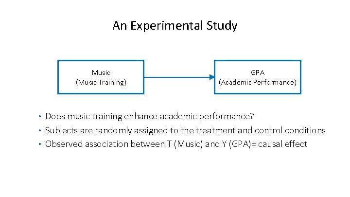
An Experimental Study Music (Music Training) GPA (Academic Performance) Does music training enhance academic performance? • Subjects are randomly assigned to the treatment and control conditions • Observed association between T (Music) and Y (GPA)= causal effect •

Establishing the Causal Effect from an Observational Study Sports Music (Music Training) GPA (Academic Performance) Observational studies: Subjects select the treatment • Observed association between T (Music) and Y (GPA) = causal effect + confounding associations •

Confounding Variables • Pretreatment characteristics that are associated with the treatment (T) and the outcome (Y) variables • Usually represented generically as common causes of T and Y • A confounding pretreatment characteristic can take two roles: v Explain parts of the treatment-outcome association v Affect the propensity of receiving treatment

Dealing with confounding pretreatment characteristics • Matching on confounding pretreatment characteristics: v Covariate matching methods v Propensity score matching and stratification methods • Adjusting for the confounding pretreatment characteristics or propensity of receiving treatment: v Weighting methods v Regression adjustment methods v Doubly robust methods

Introducing the Propensity Score Methods

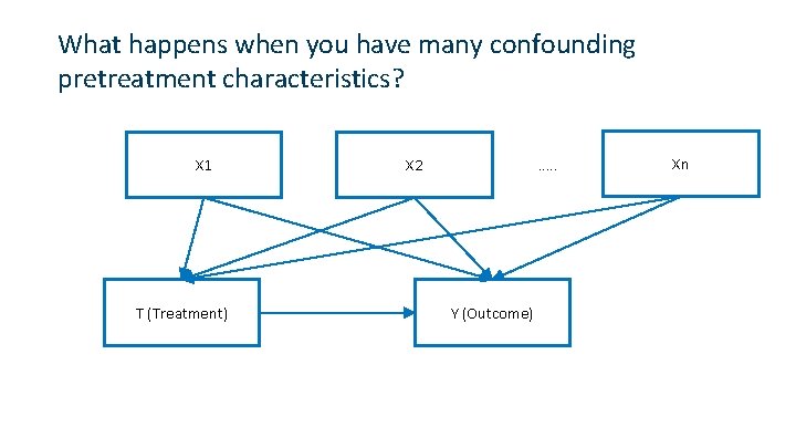
What happens when you have many confounding pretreatment characteristics? X 1 T (Treatment) …. . X 2 Y (Outcome) Xn

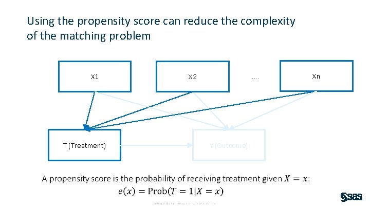
Using the propensity score can reduce the complexity of the matching problem X 1 T (Treatment) …. . X 2 Y (Outcome) Copyright © SAS Inst itute Inc. All rig hts reserved. Xn

Propensity score matching methods are … • Easier to apply than trying to match all pretreatment characteristics • Theoretical foundation: uses the potential outcomes framework to clearly define causal effects and the conditions necessary for their unbiased estimation

Example 1. Using the Optimal Matching Method of the PSMATCH Procedure

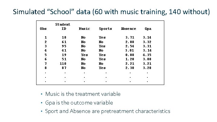
Simulated “School” data (60 with music training, 140 without) Obs 1 2 3 4 5 6 7 8. . . Student ID Music 18 61 95 41 19 51 110 87. . . No No Yes No No No. . . Sports Yes No Yes. . . Absence Gpa 3. 71 2. 08 2. 54 3. 01 0. 08 1. 20 2. 21 2. 30. . . 3. 14 3. 32 3. 31 3. 14 4. 35 3. 88 3. 21 3. 28. . . Music is the treatment variable • Gpa is the outcome variable • Sport and Absence are pretreatment characteristics •

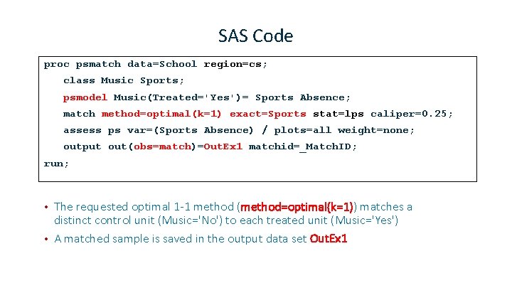
SAS Code proc psmatch data=School region=cs; class Music Sports; psmodel Music(Treated='Yes')= Sports Absence; match method=optimal(k=1) exact=Sports stat=lps caliper=0. 25; assess ps var=(Sports Absence) / plots=all weight=none; output out(obs=match)=Out. Ex 1 matchid=_Match. ID; run; The requested optimal 1 -1 method (method=optimal(k=1)) matches a distinct control unit (Music='No') to each treated unit (Music='Yes') • A matched sample is saved in the output data set Out. Ex 1 •

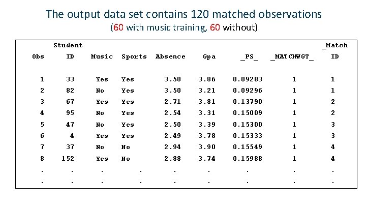
The output data set contains 120 matched observations (60 with music training, 60 without) Student _Match Obs ID Music Sports 1 33 Yes 2 82 No 3 67 4 Absence Gpa _PS_ _MATCHWGT_ ID 3. 50 3. 86 0. 09283 1 1 Yes 3. 50 3. 21 0. 09296 1 1 Yes 2. 71 3. 81 0. 13790 1 2 95 No Yes 2. 54 3. 31 0. 15009 1 2 5 47 No Yes 2. 50 3. 39 0. 15300 1 3 6 4 Yes 2. 49 3. 78 0. 15333 1 3 7 37 No No 2. 94 3. 90 0. 15549 1 4 8 152 Yes No 2. 88 3. 74 0. 15988 1 4 . . . .

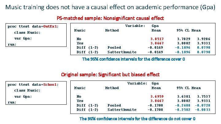
Music training does not have a causal effect on academic performance (Gpa) PS-matched sample: Nonsignificant causal effect proc ttest data=Out. Ex 1; class Music; var Gpa; run; Variable: Music No Yes Diff (1 -2) Gpa Mean Method Pooled Satterthwaite 3. 8517 3. 8667 -0. 0149 95% CL Mean 3. 7829 3. 8002 -0. 1096 3. 9206 3. 9331 0. 0798 The 95% confidence intervals for the difference cover 0 Original sample: Significant but biased effect proc ttest data=School; class Music; var Gpa; run; Variable: Music No Yes Diff (1 -2) Method Pooled Satterthwaite Gpa Mean 3. 6959 3. 8667 -0. 1708 95% CL Mean 3. 6381 3. 8002 -0. 2688 -0. 2582 3. 7537 3. 9331 -0. 0728 -0. 0833 The 95% confidence intervals for the difference do not cover 0

Theories and Assumptions

Potential outcomes framework Neyman (1923), Rubin (1974) •

The stable unit treatment value assumption (SUTVA) ensures that causal effects are well-defined (Rubin 1983) • No hidden levels of treatment • No interference among subjects

The consistency assumption relates the observed outcomes to the potential outcomes • You can observe at most one of the potential outcomes • Missing data problem: What can we know about the missing potential outcomes? •

Definitions and assumptions apply to both randomized experiments and observational studies • Same causal effect definitions by the difference in potential outcome means • Same SUTVA for defining the causal effects • Same consistency assumption about observing potential outcomes

What enables randomized experiments to obtain unbiased estimation of causal effect? •

As a consequence, for randomized experiments … •

What about observational data? •

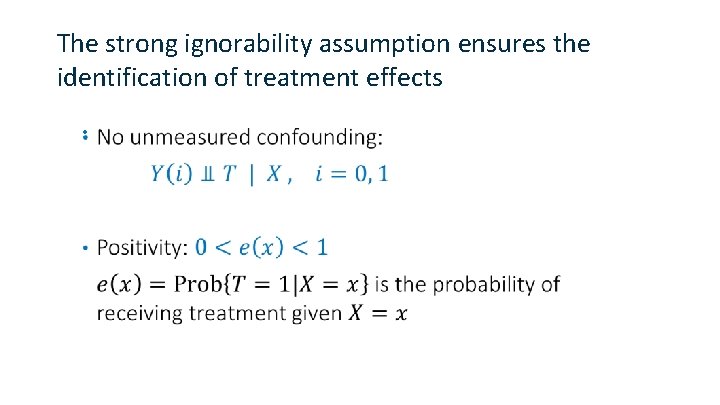
The strong ignorability assumption ensures the identification of treatment effects •

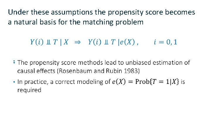
Under these assumptions the propensity score becomes a natural basis for the matching problem •

ATE or ATT? • A standard answer: ATT is for policy making • What is your research question? What is your application? v Are you interested in knowing the treatment effect if everybody in the population took the treatment? v Are you interested in knowing the treatment effect only for those who take the treatment voluntarily?

Matching aims to extract comparable groups that differ only in their treatment assignment • The ignorability assumption independence of T and potential outcomes conditional on the background characteristics • Balance in all covariates balance in propensity scores; Balance in propensity scores balance in covariates?

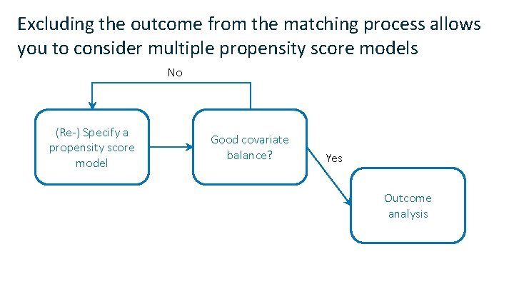
Excluding the outcome from the matching process allows you to consider multiple propensity score models No (Re-) Specify a propensity score model Good covariate balance? Yes Outcome analysis

Example 2. Optimal Variable Ratio Matching

Does quitting smoking lead to weight change? • Data: A subset (N=1, 746) of NHANES I Epidemiologic Follow-Up Study (NHEFS) in Hernán and Robins (2016) • Collect medical and behavioral information in an initial physical examination • Follow-up interviews were done approximately 10 years later • Treatment variable Quit: quit smoking during the 10 -year period • Outcome variable Change: change in weight (in kg)

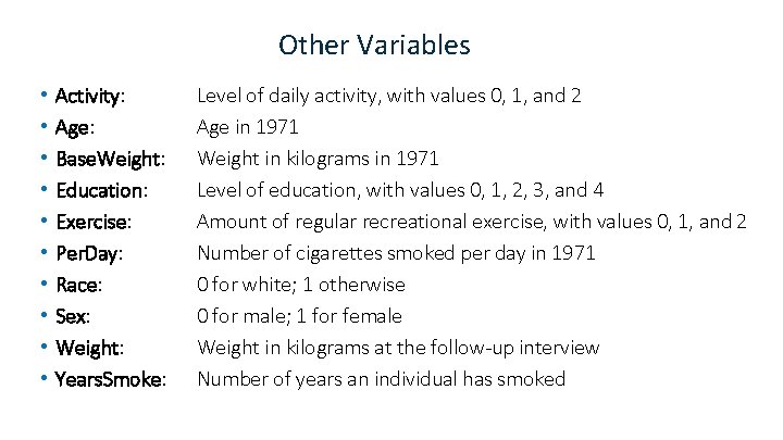
Other Variables • • • Activity: Age: Base. Weight: Education: Exercise: Per. Day: Race: Sex: Weight: Years. Smoke: Level of daily activity, with values 0, 1, and 2 Age in 1971 Weight in kilograms in 1971 Level of education, with values 0, 1, 2, 3, and 4 Amount of regular recreational exercise, with values 0, 1, and 2 Number of cigarettes smoked per day in 1971 0 for white; 1 otherwise 0 for male; 1 for female Weight in kilograms at the follow-up interview Number of years an individual has smoked

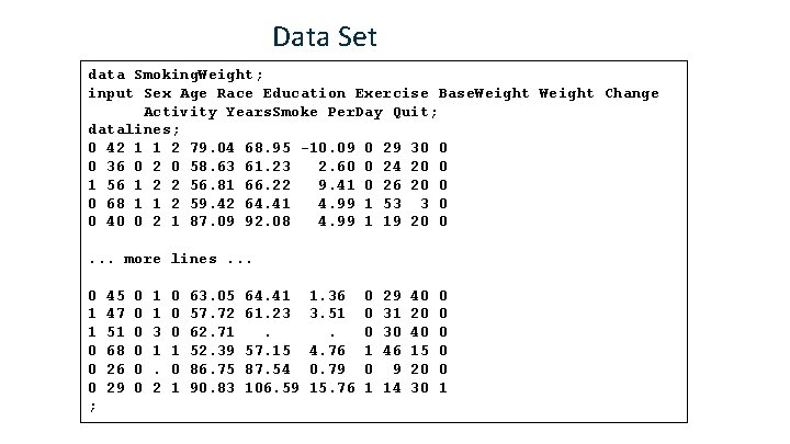
Data Set data Smoking. Weight; input Sex Age Race Education Exercise Base. Weight Change Activity Years. Smoke Per. Day Quit; datalines; 0 42 1 1 2 79. 04 68. 95 -10. 09 0 29 30 0 0 36 0 2 0 58. 63 61. 23 2. 60 0 24 20 0 1 56 1 2 2 56. 81 66. 22 9. 41 0 26 20 0 0 68 1 1 2 59. 42 64. 41 4. 99 1 53 3 0 0 40 0 2 1 87. 09 92. 08 4. 99 1 19 20 0. . . more lines. . . 0 1 1 0 0 0 ; 45 47 51 68 26 29 0 0 0 1 1 3 1. 2 0 0 0 1 63. 05 57. 72 62. 71 52. 39 86. 75 90. 83 64. 41 61. 23. 57. 15 87. 54 106. 59 1. 36 3. 51. 4. 76 0. 79 15. 76 0 0 0 1 29 31 30 46 9 14 40 20 40 15 20 30 0 0 1

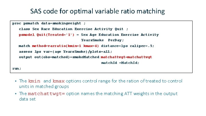
SAS code for optimal variable ratio matching proc psmatch data=smokingweight ; class Sex Race Education Exercise Activity Quit ; psmodel Quit(Treated='1') = Sex Age Education Exercise Activity Years. Smoke Per. Day; match method=varratio(kmin=1 kmax=4) distance=lps caliper=. 5; assess lps var=(age Years. Smoke)/plots=all; output out(obs=matched)=smoke. Matched matchattwgt=matchattwgt match. Id =Match. Id; run; The kmin and kmax options control range for the ration of treated to control units in matched groups • The matchattwgt= option names the matching ATT weights in the output data set •

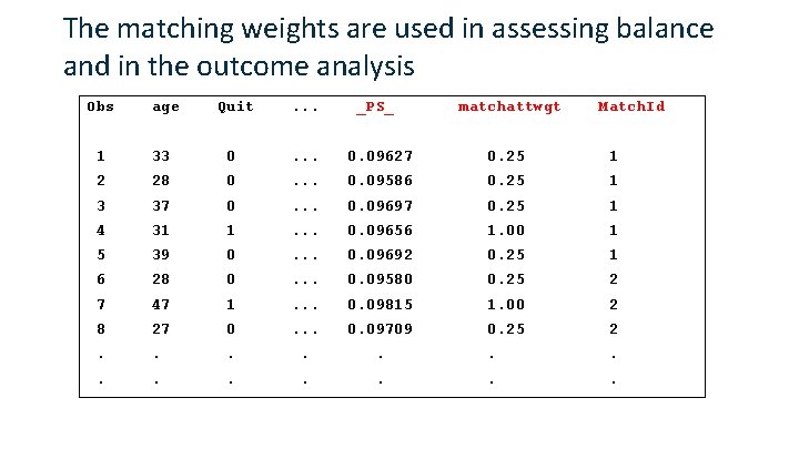
The matching weights are used in assessing balance and in the outcome analysis Obs age Quit . . . _PS_ matchattwgt Match. Id 1 33 0 . . . 0. 09627 0. 25 1 2 28 0 . . . 0. 09586 0. 25 1 3 37 0 . . . 0. 09697 0. 25 1 4 31 1 . . . 0. 09656 1. 00 1 5 39 0 . . . 0. 09692 0. 25 1 6 28 0 . . . 0. 09580 0. 25 2 7 47 1 . . . 0. 09815 1. 00 2 8 27 0 . . . 0. 09709 0. 25 2 . . .

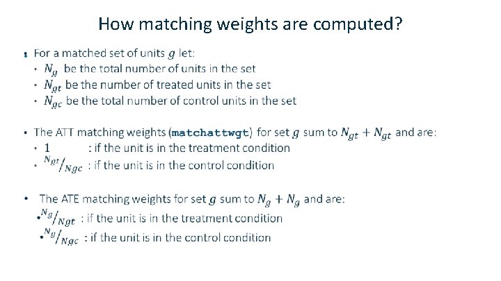
How matching weights are computed? •

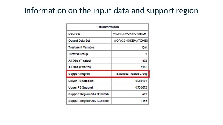
Information on the input data and support region

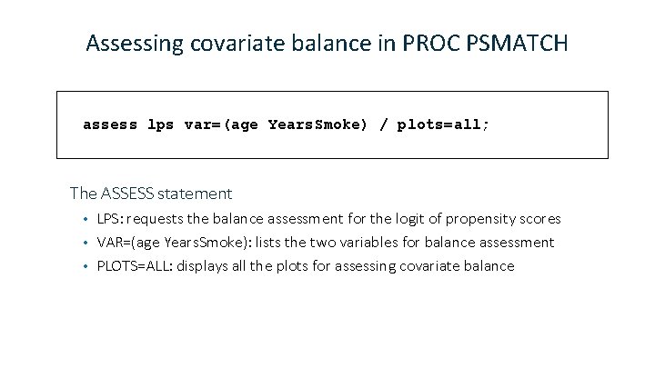
Assessing covariate balance in PROC PSMATCH assess lps var=(age Years. Smoke) / plots=all; The ASSESS statement LPS: requests the balance assessment for the logit of propensity scores • VAR=(age Years. Smoke): lists the two variables for balance assessment • PLOTS=ALL: displays all the plots for assessing covariate balance •

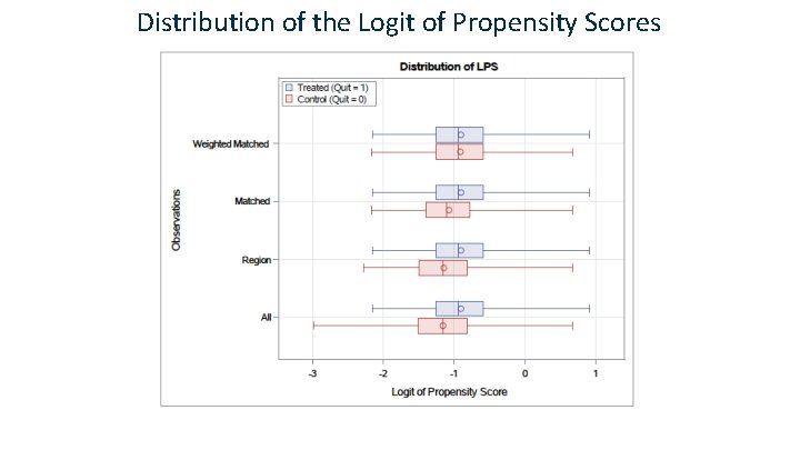
Distribution of the Logit of Propensity Scores

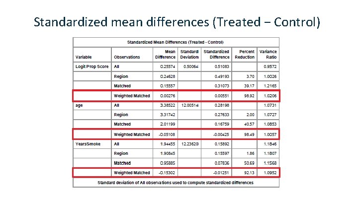
Standardized mean differences (Treated − Control)

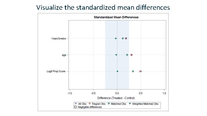
Visualize the standardized mean differences

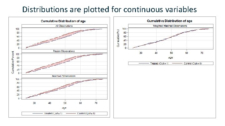
Distributions are plotted for continuous variables

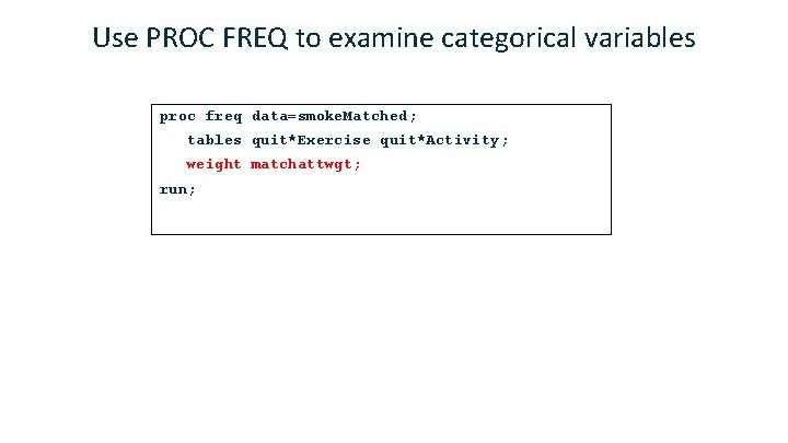
Use PROC FREQ to examine categorical variables proc freq data=smoke. Matched; tables quit*Exercise quit*Activity; weight matchattwgt; run;

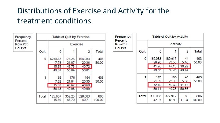
Distributions of Exercise and Activity for the treatment conditions

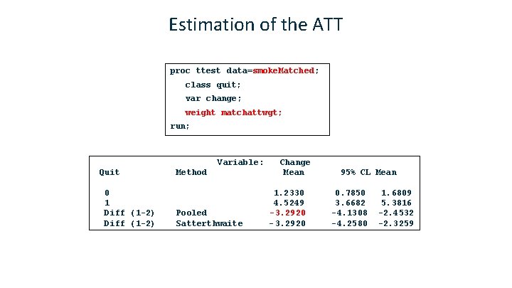
Estimation of the ATT proc ttest data=smoke. Matched; class quit; var change; weight matchattwgt; run; Variable: Quit 0 1 Diff (1 -2) Method Pooled Satterthwaite Change Mean 1. 2330 4. 5249 -3. 2920 - 3. 2920 95% CL Mean 0. 7850 3. 6682 -4. 1308 -4. 2580 1. 6809 5. 3816 -2. 4532 -2. 3259

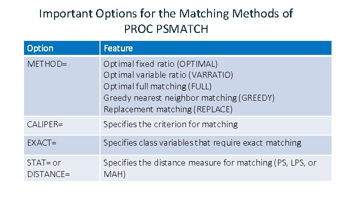
Important Options for the Matching Methods of PROC PSMATCH Option Feature METHOD= Optimal fixed ratio (OPTIMAL) Optimal variable ratio (VARRATIO) Optimal full matching (FULL) Greedy nearest neighbor matching (GREEDY) Replacement matching (REPLACE) CALIPER= Specifies the criterion for matching EXACT= Specifies class variables that require exact matching STAT= or DISTANCE= Specifies the distance measure for matching (PS, LPS, or MAH)