CAUCHY Continuity analysis of programs Swarat Chaudhuri Roberto

CAUCHY Continuity analysis of programs Swarat Chaudhuri Roberto Lublinerman Pennsylvania State University Sumit Gulwani Microsoft Research

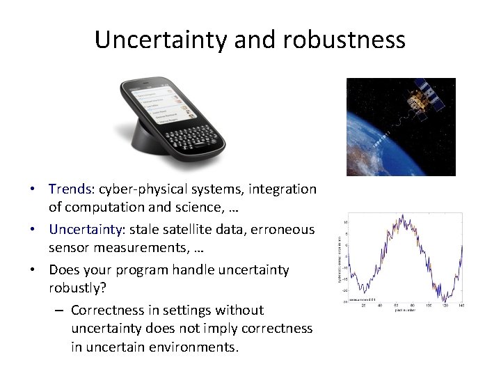
Uncertainty and robustness • Trends: cyber-physical systems, integration of computation and science, … • Uncertainty: stale satellite data, erroneous sensor measurements, … • Does your program handle uncertainty robustly? – Correctness in settings without uncertainty does not imply correctness in uncertain environments.

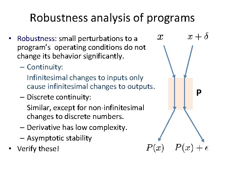
Robustness analysis of programs • Robustness: small perturbations to a program’s operating conditions do not change its behavior significantly. – Continuity: Infinitesimal changes to inputs only cause infinitesimal changes to outputs. – Discrete continuity: Similar, except for non-infinitesimal changes to discrete numbers. – Derivative has low complexity. – Asymptotic stability • Verify these! P

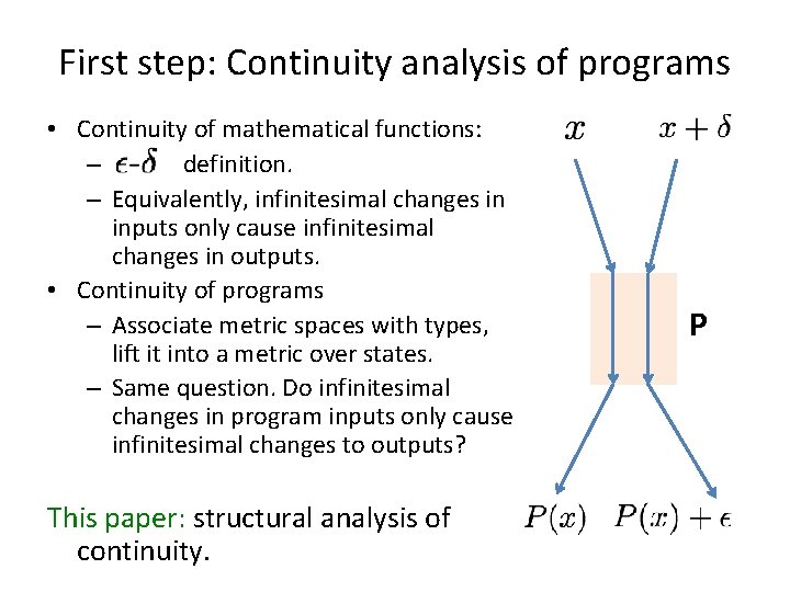
First step: Continuity analysis of programs • Continuity of mathematical functions: – definition. – Equivalently, infinitesimal changes in inputs only cause infinitesimal changes in outputs. • Continuity of programs – Associate metric spaces with types, lift it into a metric over states. – Same question. Do infinitesimal changes in program inputs only cause infinitesimal changes to outputs? This paper: structural analysis of continuity. P

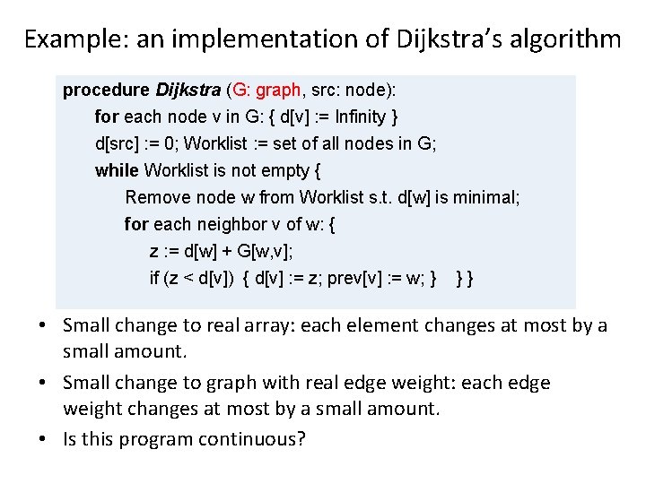
Example: an implementation of Dijkstra’s algorithm procedure Dijkstra (G: graph, src: node): for each node v in G: { d[v] : = Infinity } d[src] : = 0; Worklist : = set of all nodes in G; while Worklist is not empty { Remove node w from Worklist s. t. d[w] is minimal; for each neighbor v of w: { z : = d[w] + G[w, v]; if (z < d[v]) { d[v] : = z; prev[v] : = w; } } } • Small change to real array: each element changes at most by a small amount. • Small change to graph with real edge weight: each edge weight changes at most by a small amount. • Is this program continuous?

Example: Dijkstra’s algorithm procedure Dijkstra (G: graph, src: node): for each node v in G: { d[v] : = Infinity } d[src] : = 0; Worklist : = set of all nodes in G; while Worklist is not empty { Remove node w from Worklist s. t. d[w] is minimal; for each neighbor v of w: { z : = d[w] + G[w, v]; if (z < d[v]) { d[v] : = z; prev[v] : = w; } } } • Small change to real array: each element changes at most by a small amount. • Small change to graph • with real edge weight: each edge Depends on what is observable. weight changes at most • by a small amount. At point of output, d is a continuous function of G, but prev is not. • Is this program continuous?

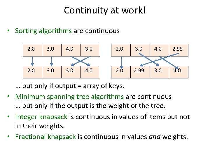
Continuity at work! • Sorting algorithms are continuous 2. 0 3. 0 4. 0 3. 0 2. 0 3. 0 4. 0 2. 99 3. 0 4. 0 … but only if output = array of keys. • Minimum spanning tree algorithms are continuous … but only if the output is the weight of the tree. • Integer knapsack is continuous in values of items but not in their weights. • Fractional knapsack is continuous in values and weights.

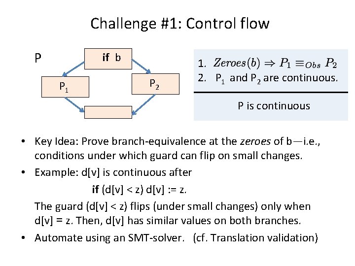
Challenge #1: Control flow P if b P 1 P 2 1. 2. P 1 and P 2 are continuous. P is continuous • Key Idea: Prove branch-equivalence at the zeroes of b—i. e. , conditions under which guard can flip on small changes. • Example: d[v] is continuous after if (d[v] < z) d[v] : = z. The guard (d[v] < z) flips (under small changes) only when d[v] = z. Then, d[v] has similar values on both branches. • Automate using an SMT-solver. (cf. Translation validation)

Challenge #2: Noninductiveness while Worklist is not empty { Remove node w from Worklist s. t. d[w] is minimal; for each neighbor v of w: { z : = d[w] + G[w, v]; if (z < d[v]) { d[v] : = z; prev[v] : = w; } u 1 d[u 1] = 2. 00 u 2 d[u 2] = 2. 00 }} u 3 d[u 2] = 4. 00 • Small change to d at iteration-entry can completely change the value of d at the end. • Thus, continuity is not inductive.

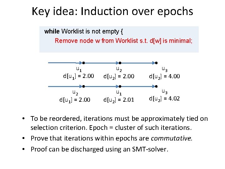
Key idea: Induction over epochs while Worklist is not empty { Remove node w from Worklist s. t. d[w] is minimal; u 1 d[u 1] = 2. 00 u 2 d[u 2] = 2. 00 u 3 d[u 2] = 4. 00 u 1 d[u 2] = 2. 01 u 3 d[u 2] = 4. 02 • To be reordered, iterations must be approximately tied on selection criterion. Epoch = cluster of such iterations. • Prove that iterations within epochs are commutative. • Proof can be discharged using an SMT-solver.

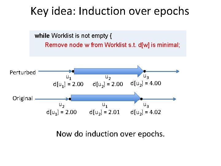
Key idea: Induction over epochs while Worklist is not empty { Remove node w from Worklist s. t. d[w] is minimal; Perturbed Original u 1 d[u 1] = 2. 00 u 2 d[u 2] = 2. 00 u 1 d[u 2] = 2. 01 u 3 d[u 2] = 4. 00 u 3 d[u 2] = 4. 02 Now do induction over epochs.

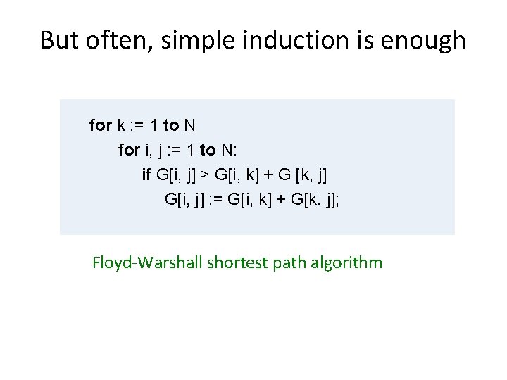
But often, simple induction is enough for k : = 1 to N for i, j : = 1 to N: if G[i, j] > G[i, k] + G [k, j] G[i, j] : = G[i, k] + G[k. j]; Floyd-Warshall shortest path algorithm

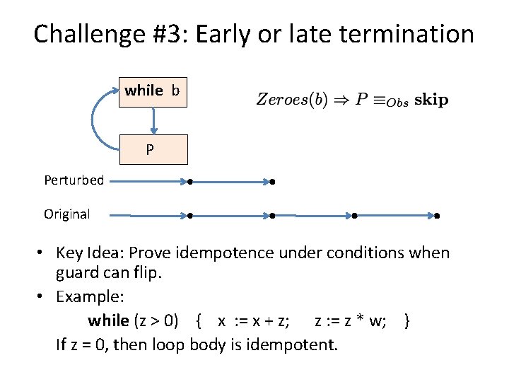
Challenge #3: Early or late termination while b P Perturbed Original • Key Idea: Prove idempotence under conditions when guard can flip. • Example: while (z > 0) { x : = x + z; z : = z * w; } If z = 0, then loop body is idempotent.

Results • Soundness with respect to definition. (Tricky!) • Proof rules discharged using Z 3 SMT solver. • Able to prove 11 of the 13 continuous algorithms targeted: – – Sorting (Merge sort, Bubble sort, Insertion sort, Selection sort). Minimum Spanning Tree (Prim’s and Kruskal’s) Shortest Paths (Floyd-Warshall, Bellman-Ford, Dijkstra) Knapsack (Fractional and integer) • Epoch induction needed in 5/13 cases. • Early termination check needed in 3/13 cases. • Current work exploring “real” applications (embedded medical devices and GPS apps).

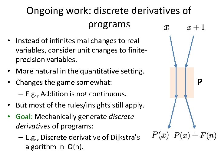
Ongoing work: discrete derivatives of programs • Instead of infinitesimal changes to real variables, consider unit changes to finiteprecision variables. • More natural in the quantitative setting. • Changes the game somewhat: – E. g. , Addition is not continuous. • But most of the rules/insights still apply. • Goal: Mechanically generate discrete derivatives of programs: – E. g. , Discrete derivative of Dijkstra’s algorithm in O(n). P

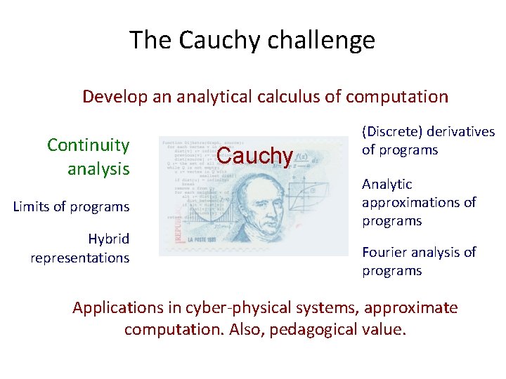
The Cauchy challenge Develop an analytical calculus of computation Continuity analysis Limits of programs Hybrid representations Cauchy (Discrete) derivatives of programs Analytic approximations of programs Fourier analysis of programs Applications in cyber-physical systems, approximate computation. Also, pedagogical value.

Conclusion • Robustness is an important correctness property for programs operating under uncertainty. • Continuity is one, but by no means the only, robustness property. • This paper offers one, but by no means the only, continuity analysis. • First step towards an analytical calculus of computation.