Categorical Data Ziad Taib Biostatistics Astra Zeneca February

Categorical Data Ziad Taib Biostatistics Astra. Zeneca February 2014

Types of Data quantitative Continuous Blood pressure Time to event Categorical sex Discrete No of relapses Ordered Categorical Pain level qualitative

Types of data analysis (Inference) Parametric Vs Non parametric Model based Vs Data driven Frequentist Vs Bayesian

Categorical data In a RCT, endpoints and surrogate endpoints can be categorical or ordered categorical variables. In the simplest cases we have binary responses (e. g. responders non-responders). In Outcomes research it is common to use many ordered categories (no improvement, moderate improvement, high improvement).

Binary variables • • Sex Mortality Presence/absence of an AE Responder/non-responder according to some pre-defined criteria • Success/Failure

Inference problems 1. Binary data (proportions) • • 2. 3. 4. 5. 6. One sample Paired data Ordered categorical data Combining categorical data Logistic regression A Bayesian alternative ODDS and NNT

Categorical data In a RCT, endpoints and surrogate endpoints can be categorical or ordered categorical variables. In the simplest cases we have binary responses (e. g. responders non-responders). In Outcomes research it is common to use many ordered categories (no improvement, moderate improvement, high improvement).

Bernoulli experiment Success 1 With probability p Random experience Failure Hole in one? 0 With probability 1 -p

Binary variables • • Sex Mortality Presence/absence of an AE Responder/non-responder according to some pre-defined criteria • Success/Failure

Estimation • Assume that a treatment has been applied to n patients and that at the end of the trial they were classified according to how they responded to the treatment: 0 meaning not cured and 1 meaning cured. The data at hand is thus a sample of n independent binary variables • The probability of being cured by this treatment can be estimated by satisfying

Hypothesis testing • We can test the null hypothesis • Using the test statistic • When n is large, Z follows, under the null hypothesis, the standard normal distribution (obs! Not when p very small or very large).

Hypothesis testing • For moderate values of n we can use the exact Bernoulli distribution of leading to the sum being Binomially distributed i. e. • As with continuous variables, tests can be used to build confidence intervals.

Example 1: Hypothesis test based on binomial distr. Consider testing against H 0: P=0. 5 Ha: P>0. 5 and where: n=10 and y=number of successes=8 p-value=(probability of obtaining a result at least as extreme as the one observed)= Prob(8 or more responders)=P 8+ P 9+ P 10= ={using the binomial formula}=0. 0547

Example 2 RCT of two analgesic drugs A and B given in a random order to each of 100 patients. After both treatment periods, each patient states a preference for one of the drugs. Result: 65 patients preferred A and 35 B

Example (cont’d) Hypotheses: H 0: P=0. 5 against H 1: P 0. 5 Observed test-statistic: z=2. 90 p-value: p=0. 0037 (exact p-value using the binomial distr. = 0. 0035) 95% CI for P: (0. 56 ; 0. 74)

Two proportions • Sometimes we want to compare the proportion of successes in two separate groups. For this purpose we take two samples of sizes n 1 and n 2. We let yi 1 and pi 1 be the observed number of subjects and the proportion of successes in the ith group. The difference in population proportions of successes and its large sample variance can be estimated by

Two proportions (continued) • Assume we want to test the null hypothesis that there is no difference between the proportions of success in the two groups (p =p ). Under the null hypothesis, we can estimate the common proportion by 11 12 • Its large sample variance is estimated by • Leading to the test statistic

Example In a trial for acute ischemic stroke *early improvement defined on a neurological scale Point estimate: 0. 080 (s. e. =0. 0397) 95% CI: (0. 003 ; 0. 158) p-value: 0. 043

Two proportions (Chi square) • The problem of comparing two proportions can sometimes be formulated as a problem of independence! Assume we have two groups as above (treatment and placebo). Assume further that the subjects were randomized to these groups. We can then test for independence between belonging to a certain group and the clinical endpoint (success or failure). The data can be organized in the form of a contingency table in which the marginal totals and the total number of subjects are considered as fixed.

2 x 2 Contingency table RESPONSE T R E A T M E N T Failure Success Total Drug 165 147 312 Placebo 190 122 312 Total 355 462 N=624

2 x 2 Contingency table RESPONSE T R E A T M E N T Failure Success Total Drug Y 10 Y 11 Y 1. Placebo Y 20 Y 21 Y 2. Total Y. 0 Y. 1 N=Y. .

Hyper geometric distribution • n balls are drawn at random without replacement. • Y is the number of white balls (successes) • Y follows the Hyper geometric Distribution with parameters (N, W, n) Urn containing W white balls and R red balls: N=W+R

Contingency tables • • • N subjects in total y. 1 of these are special (success) y 1. are drawn at random Y 11 no of successes among these y 1. Y 11 is HG(N, y. 1, y 1. ) in general

Contingency tables • The null hypothesis of independence is tested using the chi square statistic • Which, under the null hypothesis, is chi square distributed with one degree of freedom provided the sample sizes in the two groups are large (over 30) and the expected frequency in each cell is non negligible (over 5)

Contingency tables • For moderate sample sizes we use Fisher’s exact test. According to this calculate the desired probabilities using the exact Hyper-geometric distribution. The variance can then be calculated. To illustrate consider: • Using this and expectation m 11 we have the randomization chi square statistic. With fixed margins only one cell is allowed to vary. Randomization is crucial for this approach.

The (Pearson) Chi-square test 3 5 contingency table The Chi-square test is used for testing the independence between the two factors

The (Pearson) Chi-square test The test-statistic is: p where Oij = observed frequencies and Eij = expected frequencies (under independence) the test-statistic approximately follows a chi-square distribution

Example 5 Chi-square test for a 2 2 table Examining the independence between two treatments and a classification into responder/non-responder is equivalent to comparing the proportion of responders in the two groups NINDS again Observed frequencies Expected frequencies

• p 0=(122+147)/(324)=0. 43 • v(p 0)=0. 00157 which gives a p-value of 0. 043 in all these cases. This implies the drug is better than placebo. However when using Fisher’s exact test or using a continuity correction the chi square test the p-value is 0. 052.

S A S | o u t p u t

Odds, Odds Ratios and relative Risks The odds of success in group i is estimated by The odds ratio of success between the two groups i is estimated by Define risk for success in the ith group as the proportion of cases with success. The relative risk between the two groups is estimated by

Categorical data • Nominal – E. g. patient residence at end of follow-up (hospital, nursing home, own home, etc. ) • Ordinal (ordered) – E. g. some global rating • • Normal, not at all ill Borderline mentally ill Mildly ill Moderately ill Markedly ill Severely ill Among the most extremely ill patients

Categorical data & Chi-square test The chi-square test is useful for detection of a general association between treatment and categorical response (in either the nominal or ordinal scale), but it cannot identify a particular relationship, e. g. a location shift.

Nominal categorical data Chi-square test: 2 = 3. 084 , df=4 , p = 0. 544

Ordered categorical data • Here we assume two groups one receiving the drug and one placebo. The response is assumed to be ordered categorical with J categories. • The null hypothesis is that the distribution of subjects in response categories is the same for both groups. • Again the randomization and the HG distribution lead to the same chi square test statistic but this time with (J-1) df. Moreover the same relationship exists between the two versions of the chi square statistic.

The Mantel-Haensel statistic The aim here is to combine data from several (H) strata for comparing two groups drug and placebo. The expected frequency and the variance for each stratum are used to define the Mantel. Haensel statistic which is chi square distributed with one df.

Logistic regression • Consider again the Bernoulli situation, where Y is a binary r. v. (success or failure) with p being the success probability. Sometimes Y can depend on some other factors or covariates. Since Y is binary we cannot use usual regression.

Logistic regression • Logistic regression is part of a category of statistical models called generalized linear models (GLM). This broad class of models includes ordinary regression and ANOVA, as well as multivariate statistics such as ANCOVA and loglinear regression. An excellent treatment of generalized linear models is presented in Agresti (1996). • Logistic regression allows one to predict a discrete outcome, such as group membership, from a set of variables that may be continuous, discrete, dichotomous, or a mix of any of these. Generally, the dependent or response variable is dichotomous, such as presence/absence or success/failure.

Simple linear regression Table 1 Age and systolic blood pressure (SBP) among 33 adult women

SBP (mm Hg) Age (years) adapted from Colton T. Statistics in Medicine. Boston: Little Brown, 1974

Simple linear regression • Relation between 2 continuous variables (SBP and age) y Slope x • Regression coefficient 1 – Measures association between y and x – Amount by which y changes on average when x changes by one unit – Least squares method

Multiple linear regression • Relation between a continuous variable and a set of i continuous variables • Partial regression coefficients i – Amount by which y changes on average when xi changes by one unit and all the other xis remain constant – Measures association between xi and y adjusted for all other xi • Example – SBP versus age, weight, height, etc

Multiple linear regression Predicted Response variables Outcome variable Dependent variables Predictor variables Explanatory Covariables Independent

Logistic regression Table 2 Age and signs of coronary heart disease (CD)

How can we analyse these data? • Compare mean age of diseased and nondiseased – Non-diseased: 38. 6 years – Diseased: 58. 7 years (p<0. 0001) • Linear regression?

Dot-plot: Data from Table 2

Logistic regression (2) Table 3 Prevalence (%) of signs of CD according to age group

Dot-plot: Data from Table 3 Diseased % Age group

Logistic function (1) Probability of disease x

{ Transformation logit of P(y|x)

Fitting equation to the data • Linear regression: Least squares or Maximum likelihood • Logistic regression: Maximum likelihood • Likelihood function – Estimates parameters and – Practically easier to work with log-likelihood

Maximum likelihood • Iterative computing (Newton-Raphson) – Choice of an arbitrary value for the coefficients (usually 0) – Computing of log-likelihood – Variation of coefficients’ values – Reiteration until maximisation (plateau) • Results – Maximum Likelihood Estimates (MLE) for and – Estimates of P(y) for a given value of x

Multiple logistic regression • More than one independent variable – Dichotomous, ordinal, nominal, continuous … • Interpretation of i – Increase in log-odds for a one unit increase in xi with all the other xis constant – Measures association between xi and logodds adjusted for all other xi

Statistical testing • Question – Does model including given independent variable provide more information about dependent variable than model without this variable? • Three tests – Likelihood ratio statistic (LRS) – Wald test – Score test

Likelihood ratio statistic • Compares two nested models Log(odds) = + 1 x 1 + 2 x 2 + 3 x 3 (model 1) Log(odds) = + 1 x 1 + 2 x 2 (model 2) • LR statistic -2 log (likelihood model 2 / likelihood model 1) = -2 log (likelihood model 2) minus -2 log (likelihood model 1) LR statistic is a 2 with DF = number of extra parameters in model

Example 6 Fitting a Logistic regression model to the NINDS data, using only one covariate (treatment group). NINDS again Observed frequencies

S A S | o u t p u t

Logistic regression example • AZ trial (CLASS) in acute stroke comparing clomethiazole (n=678) with placebo (n=675) • Response defined as a Barthel Index score 60 at 90 days • Covariates: – – STRATUM (time to start of trmt: 0 -6, 6 -12) AGE SEVERITY (baseline SSS score) TRT (treatment group)

S A S | o u t p u t

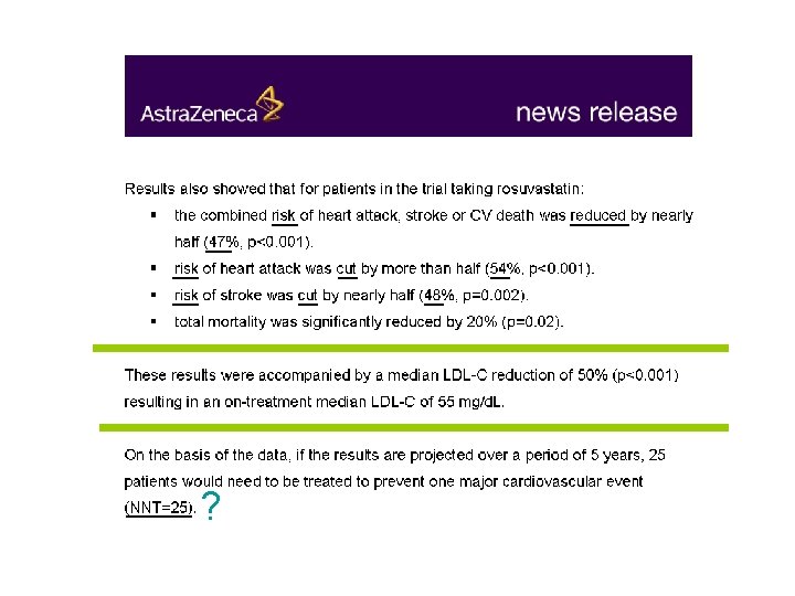
Risk Odds and NNT

David Brennan (former) CEO of Astra. Zenec

Risk, Odds and probability • Risk or chance can be measures by: – p= probabilities – O=Odds = p/(1 -p) • Probability and odds contain the same information and are equally valid as measures of chance. In case of infrequent events the distinction is unimportant. For frequent events they can be quite different.

4 measures of association (effect) – Quite often we are interested in risk and probabilty only as a way to measure association or effect: Risk is lower in the drug group = cure is associated with drug = the drug has an effect – This can be done in different ways 1. 2. 3. 4. Absolute Risk (Prospective Studies) Relative Risk (Prospective Studies) Odds Ratio (Prospective or Retrospective) (Number Needed to Treat) (Prospective Studies)

• An article in a leading medical journal reporting on a population-based case-control study of breast cancer stated that “women who used aspirin over a five-year period had a 20% reduction in breast cancer”. Here the 20% represents the relative risk, derived by • 1. 6% = risk of breast cancer reported for women who took aspirin. • 2. 0% = risk of breast cancer in women not taking aspirin. Thus, the absolute risk reduction was 2. 0% – 1. 6%% = 0. 4%, which translates to 4 fewer cases per 1, 000 women. But the relative risk reduction = 1 – 1. 6%/2. 0% = 0. 20 so the impressive 20% figure was advertised. Computations of relative risk reduction will always appear impressively large when actual event rates are low.

• • Man använder relativa tal för gynnsamma effekter, så att de ser stora ut, och absoluta tal för skadliga effekter, så att de ser små ut. Detta knep använder sig Törnberg och Nyström också av när de säger att den positiva effekten är 30 procent, medan den skadliga effekten drabbar endast 0, 1 procent av kvinnorna …… Detta är manipulation när den är som värst … » Om man undersöker 2 000 kvinnor med mammografi regelbundet i 10 år, kommer 1 av dem att ha nytta av mammografin eftersom hon kommer att undgå att dö av bröstcancer. Samtidigt kommer 10 friska kvinnor av de 2 000 deltagarna på grund av mammografin att få diagnosen bröstcancer och bli behandlade i onödan «.

The Relative Risk Versus p-value • A big relative risk does not necessarily mean that the p-value is small • The big relative risk could have occurred by chance if the sample size were small • The p-value depends both on the magnitude of the relative risk as well as the sample size.

Reciprocal fractionsare funny Relative risk: Fractions • • Assume we computed 2. 5 as the relative risk. In this calculation we divided the probability for group 1 by its counterpart for group 2. If we had divided the group 2 probability by the group 1 probability, we would have obtained a relative risk of 0. 4. This is fine because 0. 4 (2/5) and 2. 5 (5/2) are reciprocal fractions. 0. 8 (4/5) 1. 25 (5/4) 0. 75 (3/4) 1. 33 (4/3) 0. 67 (2/3) 1. 50 (3/2) 0. 50 (1/2) 2. 00 (2/1)

The scale of the odds ratios: • The variability of the odds ratio is typically based in the logarithmic scale due to assymetric character of odds ratio. 0 0. 5 1 2 OR -0. 693 0 0. 693 Log(OR) • This is especially important when deriving confidence intervals

Odds ratio vs. relative risk On Estonia: • There were 485 female passengers: 14 survived and 471 died. • There were 504 male passengers: 80 survived and 424 died n. For Alive Dead Total Female 14 471 485 Male 80 424 504 Total 94 895 989 females, the odds were 33 to 1 against surviving (471/14=33. 65). n. For males, the odds were almost 5 to 1 in favor of death (424/80=5. 3). n. The odds ratio is 0. 15 (5. 3/33. 5). There is a 6. 6 fold greater odds of death for females than for males.

• The relative risk: For females, the probability of death is 97% (471/485=0. 97). For males, the probability is 84% (424/504=0. 84). The relative risk of death is 0. 87 (0. 84/0. 97 =1/1. 15 ). There is a 1. 15 greater probability of death for females than for males. • There is quite a difference. Both measurements show that women were more likely to die. But the odds ratio (6. 6) implies that women are much worse off than the relative risk 1. 15. Which number is a fairer comparison? n. There are three issues here: –(I) The relative risk measures events in a way that is interpretable and consistent with the way “people” really think. –(II) The relative risk, though, cannot always be computed in a research design. –(III) Also, the relative risk can sometimes lead to ambiguous and confusing conclusions.

RELATIVE RISK AND ODDS RATIO • Suppose there are two groups, one with a 25% chance of mortality and the other with a 50% chance of mortality. Most people would say that the latter group has it twice as bad. But the odds ratio is 3, which seems too big. 0. 25/(1 -0. 25) / 0. 50/(1 -0. 50) = 1/3 • Even more extreme examples are possible. A change from 25% to 75% mortality represents a relative risk of 3, but an odds ratio of 9.

RELATIVE RISK vs. ODDS RATIO • • • Why would we even bother calculating the odds ratio when we can calculate relative risk? The odds ratio turns out to be important because you can calculate it either in cohort studies or case-control studies The relative risk can only be calculated from cohort studies OR can be close to the relative risk: If the disease is very rare, it is almost exactly the relative risk How rare? Rough rule of thumb: If proportion with disease is less than 1%. If disease is not rare, OR still follows same direction as RR, but may not be a very accurate estimate of RR

Number needed to treat: NNT • • NNT should be completed with follow up period and unfavourable event avoided. • NNT presupposes that there is statistically • significant difference (*). How much NNT is good? No magic figure: (10 -500) risky surgerey – standard inexpensive drug with no side effect – active treatment – preventive treatment etc. Statistical properties? Confidence intervals? When AR = 0, NNT becomes infinite! The distribution of NNT is complicated because its behaviour around AR = 0; • The moments of NNT do not exist; • Simple calculations with NNT like addition can give nonsensical results.