Categorical Data Analysis Stratified Analyses Matching and Agreement

Categorical Data Analysis: Stratified Analyses, Matching, and Agreement Statistics Biostatistics 510 13 -15 March 2007 Carla Talarico

Overview • Variable stratification • Cochran-Mantel-Haenszel (CMH) statistics • Matching and matched data • Agreement statistics – Mc. Nemar’s Test – Cohen’s Kappa

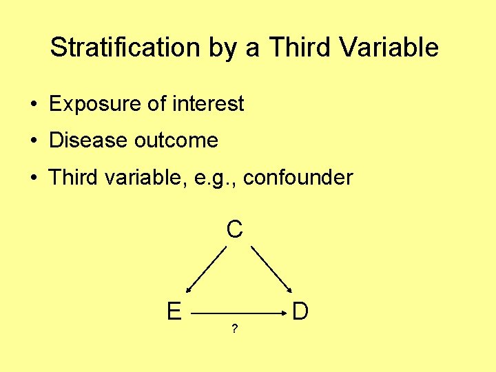
Stratification by a Third Variable • Exposure of interest • Disease outcome • Third variable, e. g. , confounder C E ? D

Confounding • Effect of exposure on disease may be different in the presence of a third variable (“Confounder”) • Reflects the fact that epidemiologic research is conducted among humans with unevenly distributed characteristics • Results because of a lack of comparability between the exposed and unexposed groups in the base population

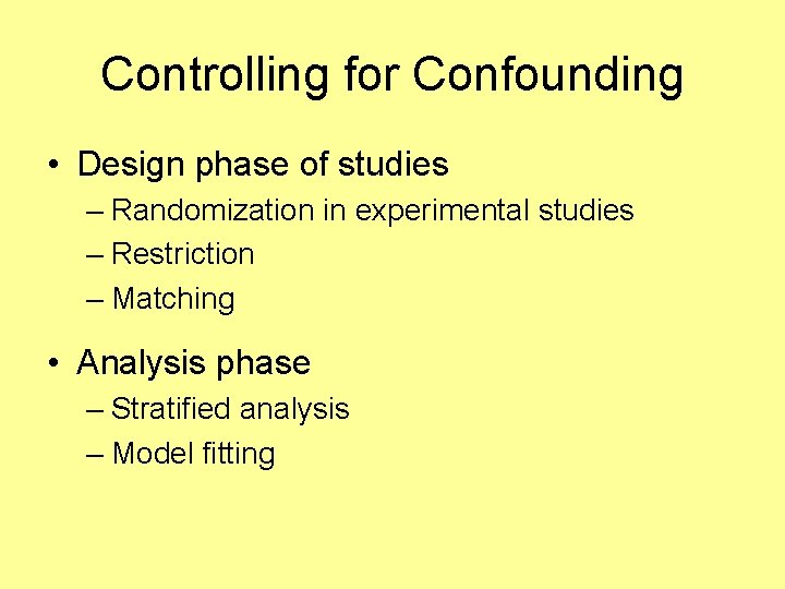
Controlling for Confounding • Design phase of studies – Randomization in experimental studies – Restriction – Matching • Analysis phase – Stratified analysis – Model fitting

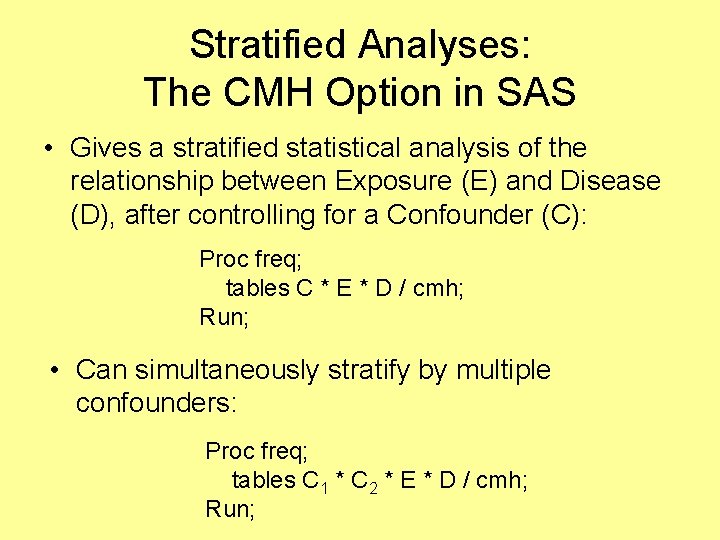
Stratified Analyses: The CMH Option in SAS • Gives a stratified statistical analysis of the relationship between Exposure (E) and Disease (D), after controlling for a Confounder (C): Proc freq; tables C * E * D / cmh; Run; • Can simultaneously stratify by multiple confounders: Proc freq; tables C 1 * C 2 * E * D / cmh; Run;

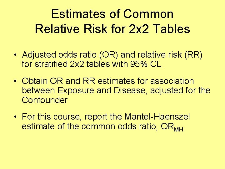
Estimates of Common Relative Risk for 2 x 2 Tables • Adjusted odds ratio (OR) and relative risk (RR) for stratified 2 x 2 tables with 95% CL • Obtain OR and RR estimates for association between Exposure and Disease, adjusted for the Confounder • For this course, report the Mantel-Haenszel estimate of the common odds ratio, ORMH

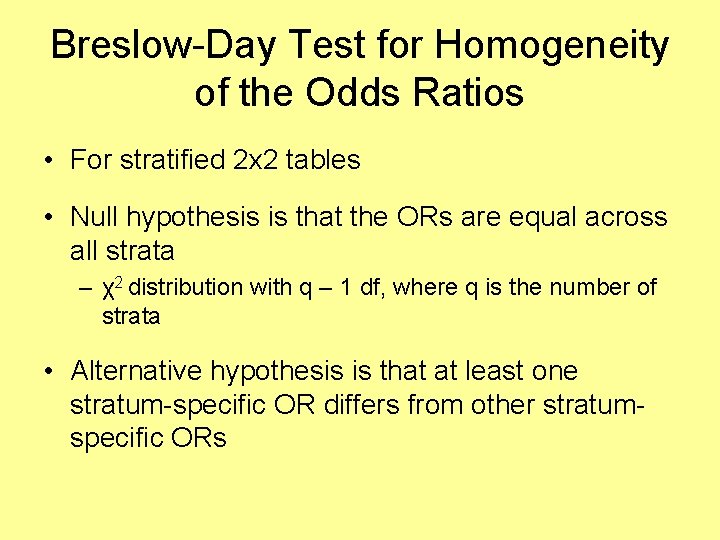
Breslow-Day Test for Homogeneity of the Odds Ratios • For stratified 2 x 2 tables • Null hypothesis is that the ORs are equal across all strata – χ2 distribution with q – 1 df, where q is the number of strata • Alternative hypothesis is that at least one stratum-specific OR differs from other stratumspecific ORs

χ2 BD (con’t) • If reject H 0 for χ2 BD test: – There is evidence for heterogeneity of ORs across strata; not appropriate to report the adjusted common OR – Report the stratum-specific ORs when effect modification is present

CMH Statistic 1: Nonzero Correlation • Tests the null hypothesis of no association vs. the alternative hypothesis that there is a linear association between the row and column variables in at least one stratum • Both row and column variables have to be ordinal • Under H 0, ~ χ2 with 1 df

CMH Statistic 2: Row Mean Scores Differ • Tests the null hypothesis of no association vs. the alternative hypothesis that the mean scores of the table rows are unequal for at least one stratum • Useful only when the column variable is ordinal • Under H 0, ~ χ2 with (r – 1) df

CMH Statistic 3: General Association • Tests the null hypothesis of no association vs. the alternative hypothesis that there is some kind of association between the row and column variables for at least one stratum • Does not require the row or column variable to be ordinal • Under H 0, ~ χ2 with (r – 1)(c – 1) df

Matching • Control for confounding more efficiently than if the matching had not been performed • Design phase of a study • Gain statistical efficiency in effect estimation

Matching (con’t) • Select comparison participants into a study such that they are the same (or nearly the same) on certain variable(s) • Matched design requires a matched analysis • Once match on a variable, the effect of that variable cannot be estimated in your data set

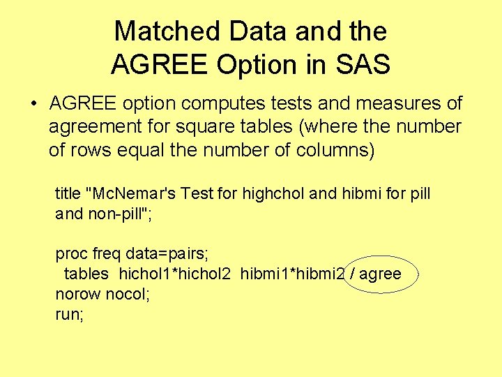
Matched Data and the AGREE Option in SAS • AGREE option computes tests and measures of agreement for square tables (where the number of rows equal the number of columns) title "Mc. Nemar's Test for highchol and hibmi for pill and non-pill"; proc freq data=pairs; tables hichol 1*hichol 2 hibmi 1*hibmi 2 / agree norow nocol; run;

AGREE Option in SAS • AGREE option generates: -Mc. Nemar’s Test -Kappa -Weighted Kappa

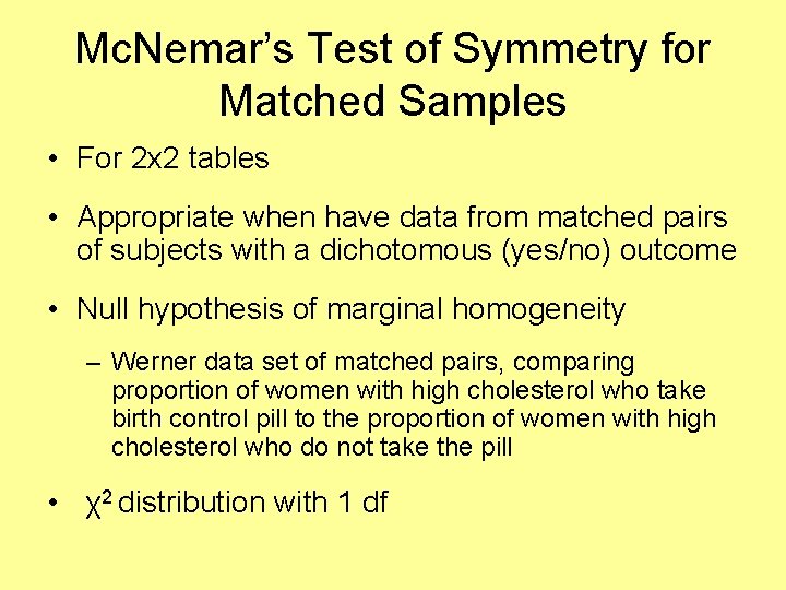
Mc. Nemar’s Test of Symmetry for Matched Samples • For 2 x 2 tables • Appropriate when have data from matched pairs of subjects with a dichotomous (yes/no) outcome • Null hypothesis of marginal homogeneity – Werner data set of matched pairs, comparing proportion of women with high cholesterol who take birth control pill to the proportion of women with high cholesterol who do not take the pill • χ2 distribution with 1 df

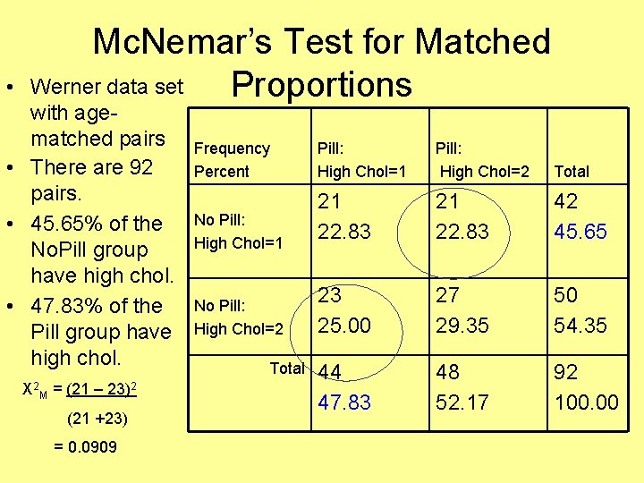
• Mc. Nemar’s Test for Matched Werner data set Proportions with agematched pairs • There are 92 pairs. • 45. 65% of the No. Pill group have high chol. • 47. 83% of the Pill group have high chol. Χ 2 M = (21 – 23)2 (21 +23) = 0. 0909 Frequency Percent No Pill: High Chol=1 No Pill: High Chol=2 Total Pill: High Chol=1 Pill: High Chol=2 Total 21 22. 83 42 45. 65 23 25. 00 27 29. 35 50 54. 35 44 47. 83 48 52. 17 92 100. 00

Simple Kappa Coefficient (Cohen’s Kappa) • Measure of inter-rater agreement, corrected for chance Κ = P 0 - P e 1 - Pe • Scale from -1 to +1 – Κ = +1 when there is perfect agreement – Κ = 0 when the agreement equals that expected by chance • Magnitude of Kappa reflects the strength of the agreement, beyond chance

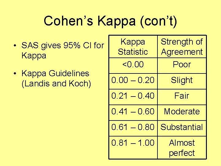
Cohen’s Kappa (con’t) • SAS gives 95% CI for Kappa • Kappa Guidelines (Landis and Koch) Kappa Statistic <0. 00 Strength of Agreement Poor 0. 00 – 0. 20 Slight 0. 21 – 0. 40 Fair 0. 41 – 0. 60 Moderate 0. 61 – 0. 80 Substantial 0. 81 – 1. 00 Almost perfect

Good Resources for Categorical Data Analysis and SAS • SAS: Categorical Data Analysis Using The SAS System by Maura E. Stokes, Charles S. Davis, and Gary G. Koch. 2 nd Ed, SAS Institute Inc. , Cary, NC, 2000. • See pages 155 -156 of Biostat 510 course pack • Kappa: “The Measurement of Observer Agreement for Categorical Data, ” by J. Richard Landis and Gary G. Koch. Biometrics 33(1): 159174, 1977