Categorical Data Analysis Chapter 4 Introduction to Generalized

Categorical Data Analysis Chapter 4: Introduction to Generalized Linear Models 1

Contents 1. 2. 3. 4. 5. 6. 7. The Generalized Linear Models for binary Data Generalized Linear Models for Counts and Rates Moments and Likelihood for Generalized Linear Models Inference and Model Checking for Generalized Linear Models Fitting Generalized Linear Models Quasi Likelihood and Generalized Linear Models 2

4. 1 : The Generalized Linear Model 3

Binomial Logit Models for Binary Data Many response variables are binary. (success and failure outcomes by 1 and 0). The Bernoulli trial has probabilities P(Y=1)=π and P(Y=0)=1 -π , for which E(Y)=π. This is the special case of the bin(1, π). 8

Poisson Loglinear Models for Count Data Some response variables have counts as their possible outcomes. The simplest distribution for count data is the Poisson. 9

Generalized Linear Models for Continuous Responses The class of GLMs also includes models for continuous responses. The normal distribution is in a natural exponential family that includes dispersion parameters. Its natural parameter is the mean. Therefore, an ordinary regression model is a GLM using the identity link. 10

Deviance of a GLM For a particular GLM for observations y=( y 1, . . . , y. N), let L(μ; y) denote the log-likelihood function expressed in terms of the means µ=(µ 1, …, µN). The deviance of a Poisson or binomial GLM is defined to be This is the likelihood-ratio statistic for testing the null hypothesis that the model holds against the general alternative (the saturated model). We use the deviance throughout the book for model checking and for inferential comparisons of models. Methods for analyzing the deviance generalize analysis of variance methods for normal linear 11 models.

Advantages of GLMs Versus Transforming the Data 1. It is not necessary that it also stabilizes variance or produces normality. 2. An advantages of GLM formulation is that the model parameters describe g[E(Y)], rather than E[g(Y)] as in the transformed data approch. 3. GLMs provide a unified theory of modeling that encompasses the most important models for continuous and discrete variables. 12

4. 2 : Generalized Linear Models For Binary Data 13

Generalized Linear Models For Binary Data Let Y denote a binary response variable, such as the result of a medical treatment(success and failure outcomes by 1 and 0), Bin(1, π). 14

Linear Probability Model For a binary response, the regression model is called a linear probability model. With independent observations it is a GLM with binomial random component and identity link function. The linear probability model has a major structural defect. Probabilities fall between 0 and 1, but linear functions take values over the entire real line. This model has π(x)<0 and π(x)>0 for some x values. The model can be valid over a restricted range of x values. When it is plausible, an advantage is its simple interpretation: βj is the 15 change in π(x) for a one-unit increase in x.

Example: Snoring and Heart Disease 16

17

Logistic Regression Model Usually, binary data result from a nonlinear relationship between π(x) and x. A fixed change in x often has less impact when π(x) is near 0 or 1 than when π(x) is near 0. 5. In practice, nonlinear relationships between π(x) and x are often monotonic , with π(x) increasing continuously or π(x) decreasing continuously as x increases. The most important curve with the S-shape has the logistic regression model formula 18

19

Logistic Regression Model Link function for logistic regression as a GLM 20

Binomial GLM for 2*2 Contingency Tables Among the simplest GLMs for a binary response is the one having a single explanatory variable X that is also binary (0, 1). 21

Probit and Inverse cdf Link Function A monotone regression curve has the shape of a cumulative distribution function (cdf) for a continuous random variable. This suggests a model for a binary response having form π (x) =F( x) for some cdf F. Using an entire class of location-scale cdf ’s, such as normal cdf ’s with their variety of means and variances, permits the curve π (x) =F( x) to have flexibility in the rate of increase and in the location where most of that increase occurs. 22

Probit and Inverse cdf Link Function Using Φ but writing the model as Replacing βx by x permits the curve to increase at a different rate than the standard cdf (or even to decrease if β<0); varying moves the curve to the left or right. When Φ is strictly increasing over the entire real line, its inverse function exists (probit model) (0, 1) (-∞, +∞) This curve has similar appearance to the logistic regression curve. 23

Latent Tolerance Motivation for Binary Response Models We now present another motivation for the link function having the form of the inverse of a cdf. For binary response models to toxicology studies, with an unobserved tolerance distribution. 24

4. 3 : Generalized Linear Models for Counts and Rates 25

Poisson Loglinear Models The Poisson distribution has a positive mean µ. Although a GLM can model a positive mean using the identity link, it is more common to model the log of the mean. Like the linear predictor , the log mean can take any real value. The log mean is the natural parameter for the Poisson distribution, and the log link is the canonical link for a Poisson GLM. A Poisson loglinear GLM assumes a Poisson distribution for Y and uses the log link. 26

Example: Horseshoe Crab Mating 27

28

29

30

Overdispersion for Poisson GLMs we noted that count data often show greater variability than the Poisson allows. For the grouped horseshoe crab data, A common cause of overdispersion is subject heterogeneity. Overdispersion is not an issue in ordinary regression with normally distributed Y, because that distribution has a separate parameter variance to describe variability. For binomial and Poisson distributions, however, the variance is a function of the mean. Overdispersion is common in the modeling of counts. 31

Negative Binomial GLMs The negative binomial distribution has probability mass function 32

Poisson Regression for Rates Using Offsets 33

Example: Modeling Death rates for Heart Valve Operations 34

Poisson GLM of Independence in Two-Way Contingency Tables 35

4. 4 : Moments and Likelihood for Generalized Linear Models 36

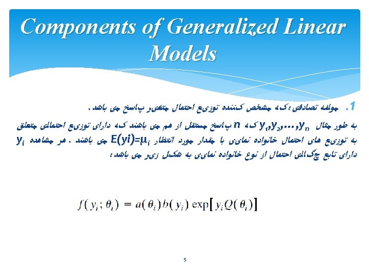
The Exponential Dispersion Family It is helpful to extend the notation for a GLM so that it can handle many distributions that have a second parameter. The random component of the GLM specifies that the N observations ( y 1, . . . , y. N ) on Y are independent, with probability mass or density function for yi of form 37

Mean and Variance Functions for the Random Component 38

Mean and Variance Functions for Poisson and Binomial GLMs When Yi is Poisson 39

Mean and Variance Functions for Poisson and Binomial GLMs When ni. Yi is bin(ni, πi) 40

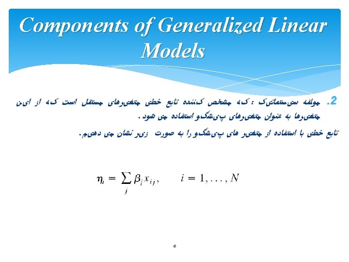
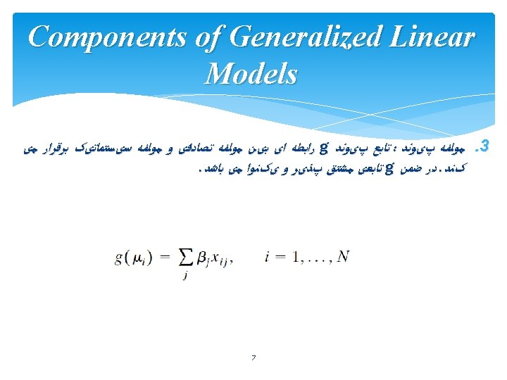
Systematic Component and Link Function of a GLM 41

Likelihood Equations for a GLM For N independent Observations (page 133) 42

Likelihood Equations for a GLM 43

The Key Role of the Mean-Variance Relationship 44

Likelihood Equations for Binomial GLMs When ni. Yi is bin(ni, πi) (Page 134) 45

Likelihood Equations for Binomial GLMs 46

Asymptotic Covariance Matrix of Model Parameter Estimators 47

Asymptotic Covariance Matrix of Model Parameter Estimators 48

Likelihood Equations and cov(β) for Poisson Loglinear Model 49

4. 5 : Inference and Model Checking for Generalized Linear Models 50

Deviance and Goodness of Fit the saturated GLM has a separate parameter for each observation. It gives a perfect fit. This sounds good, but it is not a helpful model. It does not smooth the data or have the advantages that a simpler model has, such as parsimony. Nonetheless, it serves as a baseline for other models, such as for checking model fit. 51

Deviance for Poisson GLMs For Poisson GLMs 52

Deviance for Binomial GLMs: Grouped Versus Ungrouped Data Now consider binomial GLMs with sample proportions yi based on ni trials. 53

Likelihood-Ratio Model Comparison Using The Deviances For a Poisson or binomial model M, Φ=1, so the deviance for Consider two models, M 0 with fitted values μ 0 and M 1 with fitted values µ 1, with M 0 a special case of M 1. Model M 0 is said to be nested within M 1. Since M 0 is simpler than M 1, a smaller set of parameter values satisfies M 0 than satisfies M 1. Maximizing the log likelihood over a smaller space cannot yield a larger maximum. Thus, L(µˆ 0; y)<= L(µˆ 1; y) 54

Likelihood-Ratio Model Comparison Using The Deviances Simpler models have larger deviances. Assuming that model M 1 holds, the likelihood-ratio test of the hypothesis that M 0 holds uses the test statistic The likelihood-ratio statistic comparing the two models is simply the difference between the deviances. This statistic is large when M 0 fits poorly compared to M 1. 55

Score Tests for Goodness of Fit and for Model Comparison 56

Residuals for GLMs 57

Residuals for GLMs 58

Covariance Matrices for Fitted Values and Residuals 59

Covariance Matrices for Fitted Values and Residuals 60

The Bayesian Approach for GLMs A couple of general results for GLMs are that: 61

4. 6 : Fitting Generalized Linear Models 62

Newton-Raphson Method The Newton. Raphson method is an iterative method for solving nonlinear equations, such as equations whose solution determines the point at which a function takes its maximum. 1. It begins with an initial guess for the solution. 2. It obtains a second guess by approximating the function to be maximized in a neighborhood of the initial guess by a second-degree polynomial and then finding the location of that polynomial’s maximum value. 3. It then approximates the function in a neighborhood of the second guess by another second-degree polynomial, and the third guess is the location of its maximum. 4. In this manner, the method generates a sequence of guesses. 5. These converge to the location of the maximum when the function is suitable And/or the initial guess is good. 63

Newton-Raphson Method Section 1. 3. 2 page 9 The convergence of for the Newton. Raphson method is usually fast. For large t, the convergence satisfies, for each j, 64

Fisher Scoring Method Fisher scoring is an alternative iterative method for solving likelihood equations. It resembles the Newton. Raphson method, the distinction being with the Hessian matrix. Fisher scoring uses the expected Value of this matrix, called the expected information, whereas Newton. Raphson uses the matrix itself, called the observed information. 65

Fisher Scoring Method 66

ML as Iterative Reweighted Least Squares A relation exists between weighted least squares estimation and using Fisher scoring to find ML estimates. For the general linear model of form 67

ML as Iterative Reweighted Least Squares 68

ML as Iterative Reweighted Least Squares 69

Simplifications for Canonical Link Functions 70

Simplifications for Canonical Link Functions 71

4. 7 : Quasi-Likelihood and Generalized Linear Models 72

Mean-Variance Relationship Determines Quasi-Likelihood Estimates The likelihood equation Wedderburn proposed an alternative approach, quasi-likelihood estimation, which assumes only a mean variance relationship rather than a specific distribution for Yi. It has a link function and linear predictor of the usual GLM form, but instead of assuming a distributional type for Yi it assumes only The quasi-likelihood QL estimates are with v(µi ) replaced by µi. Under the additional assumption that Yi have distribution in the natural exponential, these estimates are also ML estimates. That case is simply the Poisson distribution. Thus, for v(µ)= µ, quasi-likelihood estimates are also ML estimates when the random component has a Poisson distribution. 73

Overdispersion for Poisson GLMs and Quasi-Likelihood For count data, we’ve seen that the Poisson assumption is often unrealistic because of overdispersion the variance exceeds the mean. One cause for this is heterogeneity among subjects. This suggests an alternative to a Poisson GLM in which the mean variance relationship has the form for some constant Φ. The case Φ > 1 represents overdispersion for the Poisson model. In the estimating equations with , Φ drops out. Thus, the equations are identical to likelihood equations for Poisson models, and model parameter estimates are also identical. Also, 74

Overdispersion for Binomial GLMs and Quasi-Likelihood 75

Example: Teratology Overdispersion 76

Thanks For Your Consideration Spring 2014 77