Carbonate sediment supply on oceanic islands A model

Carbonate sediment supply on oceanic islands: A model and its applications Jodi N. Harney Charles H. Fletcher University of Hawaii Dept. of Geology and Geophysics

OUTLINE © Introduction, objectives, and approach in Kailua Bay, Oahu © Methods Substrate mapping ³ Physiographic zonation ³ Sediment production ³ © Applications © Conclusions

Sediment Budgets Quantitative estimates of sources, sinks, fluxes, losses of sediment within a defined system • among primary controls of coastal morphology and evolution • affects development of beaches, dunes, reefs • can be instrumental in predicting and interpreting coastal behavior

Beaches in Hawaii (Moberly et al. 1965) Dark detrital grains derived from volcanic rocks Calcareous skeletal remains of reef-dwelling organisms Relative proportion varies with local conditions

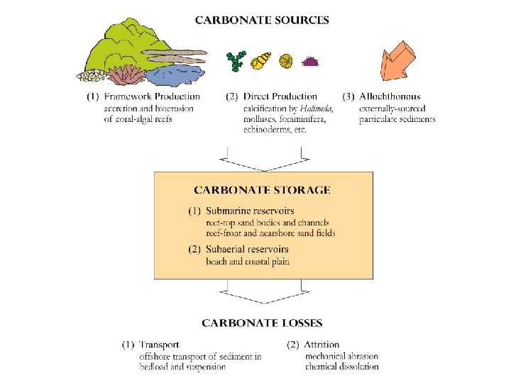
On oceanic islands in low latitudes, calcareous sediment supply is controlled by shallow-marine carbonate productivity (reefs and associated settings)

Kailua Bay, Oahu ð carbonate reef complex 0– 25 m water depth ð 200 -m wide paleostream channel bisects platform ð seaward mouth opens onto 30– 70 m deep sand field ð high-resolution central portion is MS imagery

Multispectral imagery (Isoun et al. 199

Sediment composition and age Harney et al. 2000. Coral Reefs 19: 141– 154.

Approach © Map distribution and abundance of carbonate producers across the reef complex © Define physiographic zones in terms of benthic communities © Measure Ca. CO 3 production rates of sedimentproducing organisms © Calculate annual sediment production

Substrate Mapping Line transect method Each transect map provides >50 variables that describe: • distribution and abundance of substrate types (rubble, sand, dead coral, living coral, coralline algae, Halimeda) • reef topography (rugosity) • community structure • species composition • growth form 52 sites mapped in Kailua Bay

Physiographic zones ³ each with a suite of biogeological characteristics based on mapping data collected within zone ³ zone area measured using image analysis software and corrected for reef rugosity

Measuring coral growth and bioerosion GPRe = 2. 8 kgm-2 y-1 GPRfb = 10. 7 kgm-2 y-1 GPRm = 8. 4 kgm-2 y-1 Bioerosion (Bz) = 0. 2– 1 kgm-2 y-1 Rates consistent with those published for Hawaiian reefs (e. g. Grigg 1995)

Measuring standing crop of direct producers Halimeda GPRHo = 6. 5 kgm-2 y-1 Benthic forams (and micromolluscs) GPRF = 0. 1– 0. 4 kgm-2 y-1 Clear plants from a measured area of seafloor; remove organic matter; measure Ca. CO 3 content in kgm-2 Collect samples of rubble; remove living organisms; measure Ca. CO 3 content in kgm-2 GPRM = 0. 1– 0. 4 kgm-2 y-1 Articulated coralline algae GPRapg = 10 kgm-2 y-1 Collect individual living clumps; remove organic matter; measure Ca. CO 3 content in kgm-2 Rates consistent with those in literature

Rates of Ca. CO 3 production and erosion Gross Production Rates (kgm-2 y-1): Direct Production Rates (kgm-2 y-1): 2. 8 = GPRe (encrusting coral) 0. 3– 3. 0 = GPRHd Halimeda discoidea 8. 4 = GPRm (massive coral) 6. 4– 6. 7 = GPRHo Halimeda opuntia 6. 7 = GPRsb (stout-branching coral) 0. 05– 1. 8 = GPRM micromolluscs (finger-branching coral) 0. 05– 0. 1 = GPRF benthic forams (encrust. coralline algae) 10. 0– 17. 8 = GPRapg articulated coralline algae 10. 7 = GPRfb 2. 6 = GPRace 0. 2– 1. 0 = Bz (bioerosion rate by zone) Sources include: Grigg 1982, 1995, 1998; Agegian 1985 Comparable to data from sources including: Drew & Abel 1985, Payri 1988, Hillis 1997 (Halimeda) Hallock 1981, 1984 (forams) Agegian 1985 (artic. coralline algae)

Organism abundance by zone For each zone, mapping data is pooled and averaged: Habitat area (m 2) Rugosity (expresses reef topography, R = 1– 4) Percent living coral cover: Ce encrusting Cm massive Csb stout-branching Cfb finger-branching (Porites lobata, Montipora patula, M. verrucosa) (Porites lobata) (Pocillopora meandrina) (Porites compressa) Percent coralline algae cover: Cace encrusting (Porolithon onkodes and others) Capg articulated (Porolithon gardineri) Percent Halimeda cover: CHd H. discoidea CHo H. opuntia

Equations for gross framework production For each zone: Habitat area (m 2) Ah = A s R Gross production by coral (each growth form: e, m, sb, fb) Ge = Ce Ah GPRe Gross production by all coral forms Gc = Ge + Gm + Gsb + Gfb Gross production by encrusting coralline algae Gace = Cace Ah GPRace Total unconsolidated sediment produced by bioerosion of reef framework (kgy-1) SF = (Gc + Gace) Bz

Equations for direct sediment production For each zone: Habitat area (m 2) Ah = A s R Direct production by Halimeda SH = CH Ah GPRH Direct production by forams SF = CF Ah GPRF Direct production by micromolluscs SM = CM Ah GPRM Direct production by articulated coralline algae Sapg = Capg Ah GPRapg Sum of all direct sediment production sources SD = SH + SF + SM + Sapg TOTAL sediment production (kgy-1) ST = S F + SD

Sediment production by zone Nearshore hardgrounds (NH) SF = 121 x 103 kgy-1 0. 19 kgm-2 y-1 SD = 110 x 104 kgy-1 1. 81 kgm-2 y-1 Coral garden (SCG) SF = 34 x 103 kgy-1 0. 39 kgm-2 y-1 SD = 1. 5 x 103 kgy -1 0. 01 kgm-2 y-1 Seaward reef platform (S 1) SF = 329 x 103 kgy-1 0. 35 kgm-2 y-1 SD = 142 x 103 kgy-1 0. 13 kgm-2 y-1 Rate of sediment production by Kailua reef complex = Range 0. 3 – 2. 0 kgm-2 y-1 Avg. 0. 86 kgm-2 y-1 (~700 cm 3)

Total Sediment Production SF = 2982 ± 179 x 103 kgy-1 SD = 4498 ± 565 x 103 kgy-1 ST = 7480 ± 744 x 103 kgy-1 (average = 0. 86 kgm-2 y-1 ) convert to volume ASV = 7039 ± 1172 m 3 y-1 Annual Sediment Volume

Applications Holocene sediment budget, Kailua Bay Total Holocene Sediment Production 35196 ± 5862 x 103 m 3 Total Sediment Storage 14375 ± 2174 x 103 m 3 Sediment Lost 20821 ± 8036 x 103 m 3 (or unaccounted for) 41 (± 7) % 59 (± 7) %

Coastal and carbonate dynamics Total calcareous sediment production 7039 ± 1172 m 3 y-1 Per reef surface area = 0. 0007 m 3 m-2 y-1 41% stays in system, 4% goes to beach Annual beach replenishment = 115 m 3 y-1 rate 43 m 3 m-1 beach length Net seasonal shoreline change, = 172, 000 m 3 annual flux Kailua Beach (Gibbs et al. 2000) Difference in rates of beach supply and shoreline change is 3 orders of magnitude

HANALEI, KAUAI Holocene Shoreline Progradation • 5000 year carbonate sediment supply = 21. 5 x 106 m 3 • Holocene progradation history required additional calcareous sediment supplied by transport from Anini reef: 3760 m 3 each year for 5000 years = 18. 8 x 106 m 3

KIHEI, MAUI Shoreline Change • Erosion along the south Kihei coast is linked to the northward transport of coastal sediments • In the last century, a volume equivalent to 1600 years of carbonate sediment production has migrated from south Kihei northward

LANIKAI, OAHU Beach Renourishment + 12, 000 m 3 Kailua SS = 7039 m 3 y-1 System = 41% of budget Beach = 4% of budget Replacement rate ~ 115 m 3 y-1 Replacement time ~ 100 y

CONCLUSIONS © Carbonate sediment supply is an important factor in the behavior and evolution of coastal margins; depends on reef productivity; can be estimated using a field-based model © Annual rates of sediment supply are instrumental in developing sediment budgets and understanding coastal behavior over space and time © In Kailua, carbonate sediments are produced at a rate of 7039 ± 1172 m 3 y-1; 41% of those produced in the last 5000 years remain stored in bay and coastal plain © The Kailua model is the most comprehensive, fieldbased effort on the largest system to date; first for Hawaii; can be applied to other reef systems © Rates at which reefs produce sediment are slow compared to rates of shoreline change

Mahalo