Capital Market Theory and Asset Pricing Models Chapter

Capital Market Theory and Asset Pricing Models Chapter 9 Charles P. Jones, Investments: Analysis and Management, Twelfth Edition, John Wiley & Sons 91

Capital Asset Pricing Model Positive rather than normative ◦ Describes how investors could behave not how they should be have Focus on the equilibrium relationship between the risk and expected return on risky assets Builds on Markowitz portfolio theory Each investor is assumed to diversify his or her portfolio according to the Markowitz model 92

Assumes all investors: ◦ Use the same information to generate an efficient frontier ◦ Have the same oneperiod time horizon ◦ Can borrow or lend money at the risk-free rate of return No transaction costs, no personal income taxes, no inflation No single investor can affect the price of a stock Capital markets are in equilibrium 93

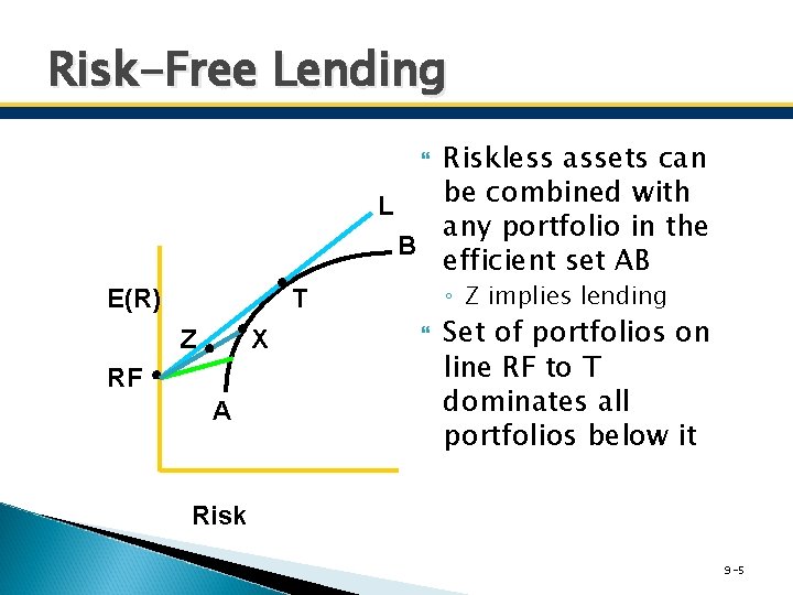
Risk-Free Assets, Borrowing, Lending Risk free assets ◦ No correlation with risky assets ◦ Usually proxied by a Treasury security Adding a risk-free asset extends and changes the efficient frontier “Lending” because investor lends money to issuer With borrowing, investor no longer restricted to own wealth 94

Risk-Free Lending Riskless assets can be combined with L any portfolio in the B efficient set AB E(R) ◦ Z implies lending T Z X RF A Set of portfolios on line RF to T dominates all portfolios below it Risk 9 -5

The New Efficient Set Risk-free investing and borrowing creates a new set of expected return-risk possibilities Addition of risk-free asset results in ◦ A change in the efficient set from an arc to a straight line tangent to the feasible set without the riskless asset ◦ Chosen portfolio depends on investor’s risk-return preferences 96

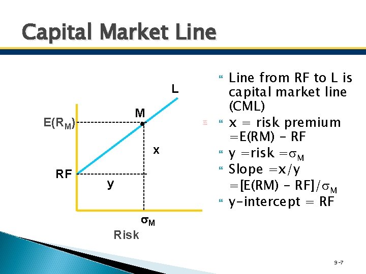
Capital Market Line L M E(RM) x RF y M Line from RF to L is capital market line (CML) x = risk premium =E(RM) - RF y =risk = M Slope =x/y =[E(RM) - RF]/ M y-intercept = RF Risk 9 -7

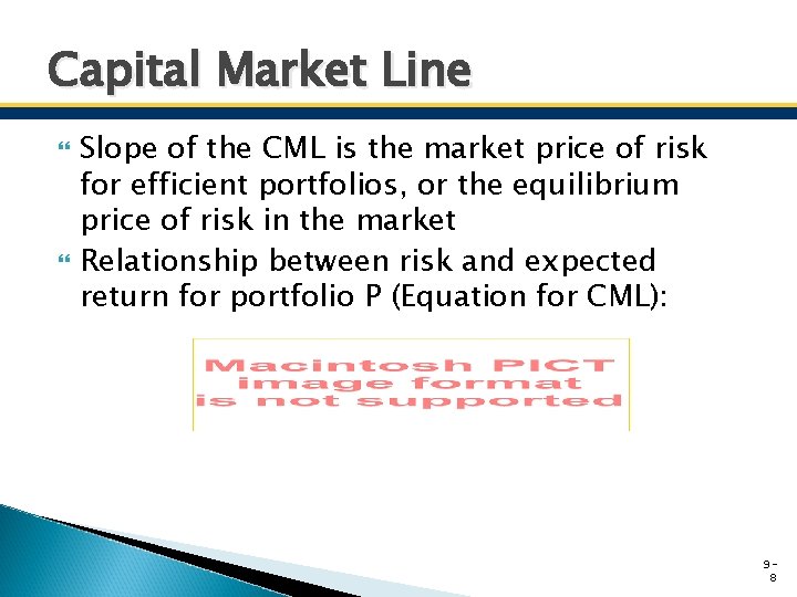
Capital Market Line Slope of the CML is the market price of risk for efficient portfolios, or the equilibrium price of risk in the market Relationship between risk and expected return for portfolio P (Equation for CML): 98

Market Portfolio Most important implication of the CAPM ◦ The portfolio of all risky assets is the optimal risky portfolio (called the market portfolio) ◦ The expected price of risk is always positive ◦ The optimal portfolio is at the highest point of tangency between RF and the efficient frontier ◦ All investors hold the same optimal portfolio of risky assets 99

Characteristics of the Market Portfolio All risky assets must be in portfolio, so it is completely diversified ◦ Includes only systematic risk Unobservable but approximated with portfolio of all common stocks ◦ In turn approximated with S&P 500 All securities included in proportion to their market value 910

The Separation Theorem Investors use their preferences (reflected in an indifference curve) to determine optimal portfolio Separation Theorem ◦ The investment decision about which risky portfolio to hold is separate from the financing decision Investment decision does not involve investor Financing decision depends on investor’s preferences 911

Security Market Line CML Equation only applies to markets in equilibrium and efficient portfolios The Security Market Line depicts tradeoff between risk and expected return for individual securities Under CAPM, all investors hold the market portfolio ◦ Relevant risk of any security is therefore its covariance with the market portfolio 912

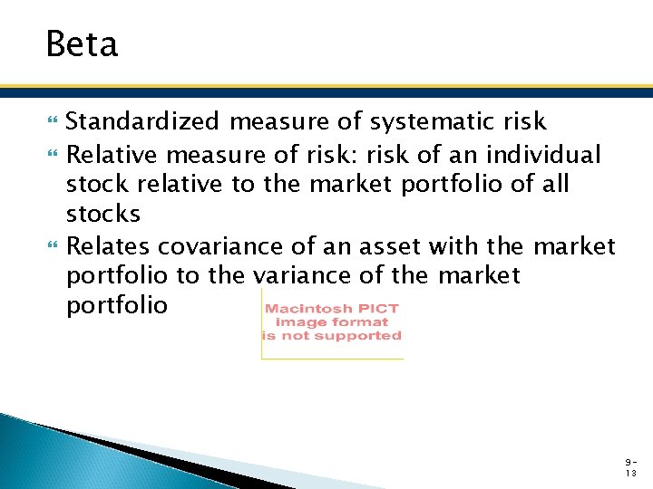
Beta Standardized measure of systematic risk Relative measure of risk: risk of an individual stock relative to the market portfolio of all stocks Relates covariance of an asset with the market portfolio to the variance of the market portfolio 913

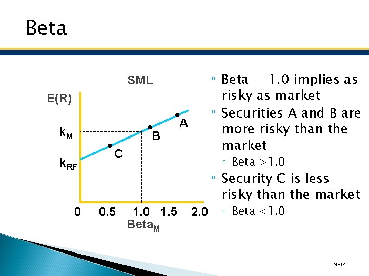
Beta SML E(R) k. M B k. RF A C ◦ Beta >1. 0 0 0. 5 Beta = 1. 0 implies as risky as market Securities A and B are more risky than the market 1. 0 1. 5 Beta. M 2. 0 Security C is less risky than the market ◦ Beta <1. 0 9 -14

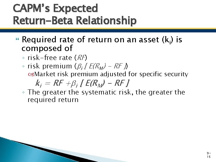
CAPM’s Expected Return-Beta Relationship Required rate of return on an asset (ki) is composed of ◦ risk-free rate (RF) ◦ risk premium ( i [ E(RM) - RF ]) Market risk premium adjusted for specific security ki = RF + i [ E(RM) - RF ] ◦ The greater the systematic risk, the greater the required return 915

Estimating the SML Treasury Bill rate used to estimate RF Expected market return unobservable ◦ Estimated using past market returns and taking an expected value Estimating individual security betas difficult ◦ Only company-specific factor in CAPM ◦ Requires asset-specific forecast 916

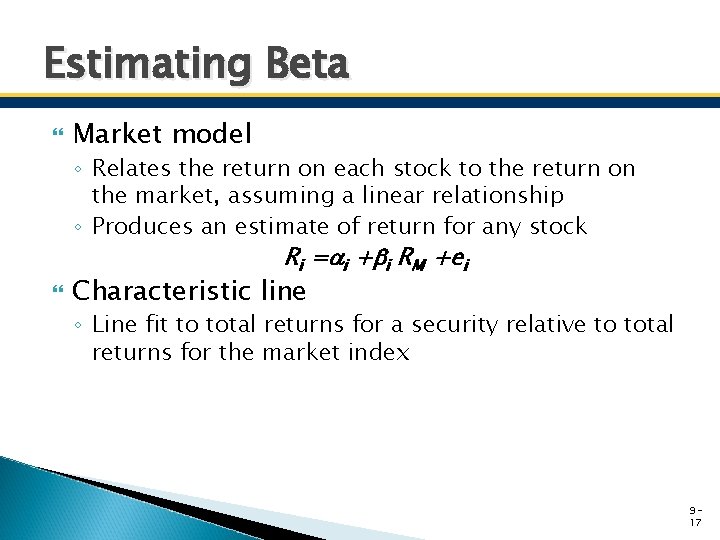
Estimating Beta Market model ◦ Relates the return on each stock to the return on the market, assuming a linear relationship ◦ Produces an estimate of return for any stock Ri = i + i RM +ei Characteristic line ◦ Line fit to total returns for a security relative to total returns for the market index 917

How Accurate Are Beta Estimates? Betas change with a company’s situation Estimating a future beta ◦ May differ from the historical beta RM represents the total of all marketable assets in the economy ◦ Approximated with a stock market index ◦ Approximates return on all common stocks 918

How Accurate Are Beta Estimates? No one correct number of observations and time periods for calculating beta ◦ Therefore, estimates of beta vary The regression calculations of the true and from the characteristic line are subject to estimation error Portfolio betas more reliable than individual security betas 919

Tests of CAPM Assumptions are mostly unrealistic Empirical evidence has not led to consensus However, some points are widely agreed upon ◦ SML appears to be linear ◦ Intercept is generally higher than RF ◦ Slope of the CAPM is generally less than theory predicts ◦ It’s likely that only systematic risk is rewarded 920

Arbitrage Pricing Theory Based on the Law of One Price ◦ Two otherwise identical assets cannot sell at different prices ◦ Equilibrium prices adjust to eliminate all arbitrage opportunities Unlike CAPM, APT does not assume ◦ single-period investment horizon, absence of personal taxes, riskless borrowing or lending, mean -variance decisions 921

Factors APT assumes returns generated by a factor model Factor Characteristics ◦ Each risk must have a pervasive influence on stock returns ◦ Risk factors must influence expected return and have non-zero prices ◦ Risk factors must be unpredictable to the market 922

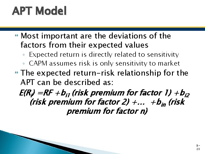
APT Model Most important are the deviations of the factors from their expected values ◦ Expected return is directly related to sensitivity ◦ CAPM assumes risk is only sensitivity to market The expected return-risk relationship for the APT can be described as: E(Ri) =RF +bi 1 (risk premium for factor 1) +bi 2 (risk premium for factor 2) +… +bin (risk premium for factor n) 923

Problems with APT Factors are not well specified ex ante ◦ To implement the APT model, need the factors that account for the differences among security returns CAPM identifies market portfolio as single factor Studies suggest certain factors are reflected in market ◦ Focus on cash flows and discount rate Both CAPM and APT rely on unobservable expectations 924

Copyright 2013 John Wiley & Sons, Inc. All rights reserved. Reproduction or translation of this work beyond that permitted in section 117 of the 1976 United States Copyright Act without express permission of the copyright owner is unlawful. Request for further information should be addressed to the Permissions Department, John Wiley & Sons, Inc. The purchaser may make backup copies for his/her own use only and not for distribution or resale. The Publisher assumes no responsibility for errors, omissions, or damages caused by the use of these programs or from the use of the information herein. 925