Capital Asset Pricing and Arbitrage Pricing Theory Bodie

Capital Asset Pricing and Arbitrage Pricing Theory Bodie, Kane, and Marcus Essentials of Investments, 9 th Edition Mc. Graw-Hill/Irwin 7 Copyright © 2013 by The Mc. Graw-Hill Companies, Inc. All rights reserved.

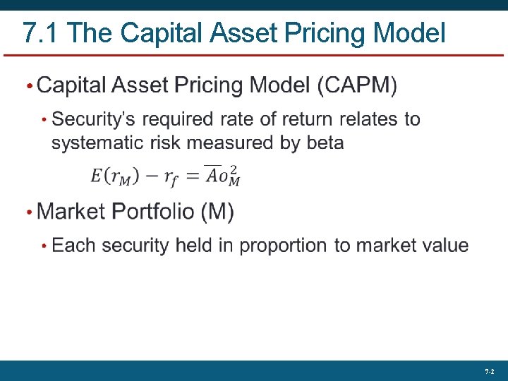
7. 1 The Capital Asset Pricing Model • 7 -2

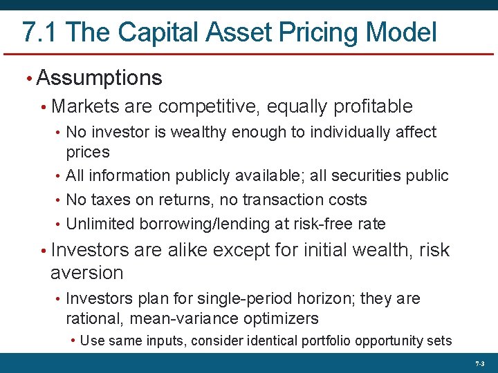
7. 1 The Capital Asset Pricing Model • Assumptions • Markets are competitive, equally profitable • No investor is wealthy enough to individually affect prices • All information publicly available; all securities public • No taxes on returns, no transaction costs • Unlimited borrowing/lending at risk-free rate • Investors are alike except for initial wealth, risk aversion • Investors plan for single-period horizon; they are rational, mean-variance optimizers • Use same inputs, consider identical portfolio opportunity sets 7 -3

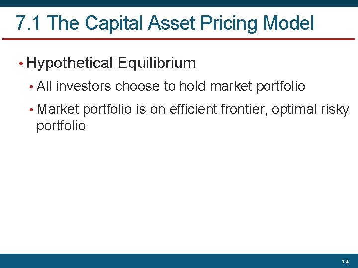
7. 1 The Capital Asset Pricing Model • Hypothetical Equilibrium • All investors choose to hold market portfolio • Market portfolio is on efficient frontier, optimal risky portfolio 7 -4

7. 1 The Capital Asset Pricing Model • Hypothetical Equilibrium • Risk premium on market portfolio is proportional to variance of market portfolio and investor’s risk aversion • Risk premium on individual assets • Proportional to risk premium on market portfolio • Proportional to beta coefficient of security on market portfolio 7 -5

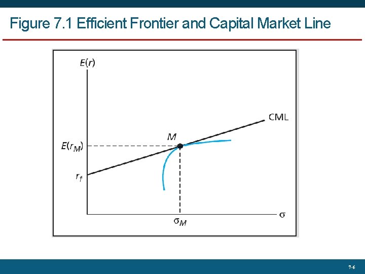
Figure 7. 1 Efficient Frontier and Capital Market Line 7 -6

7. 1 The Capital Asset Pricing Model • Passive Strategy is Efficient • Mutual fund theorem: All investors desire same portfolio of risky assets, can be satisfied by single mutual fund composed of that portfolio • If passive strategy is costless and efficient, why follow active strategy? • If no one does security analysis, what brings about efficiency of market portfolio? 7 -7

7. 1 The Capital Asset Pricing Model • Risk Premium of Market Portfolio • Demand drives prices, lowers expected rate of return/risk premiums • When premiums fall, investors move funds into risk-free asset • Equilibrium risk premium of market portfolio proportional to • Risk of market • Risk aversion of average investor 7 -8

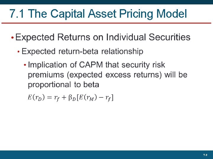
7. 1 The Capital Asset Pricing Model • 7 -9

7. 1 The Capital Asset Pricing Model • The Security Market Line (SML) • Represents expected return-beta relationship of CAPM • Graphs individual asset risk premiums as function of asset risk • Alpha • Abnormal rate of return on security in excess of that predicted by equilibrium model (CAPM) 7 -10

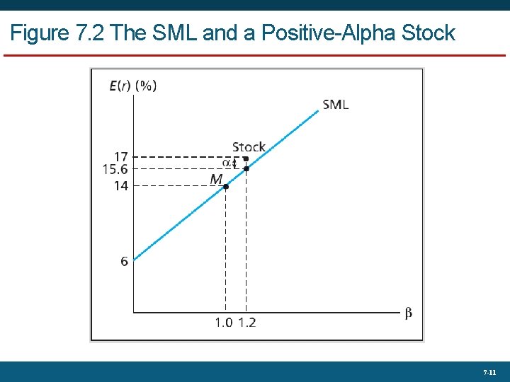
Figure 7. 2 The SML and a Positive-Alpha Stock 7 -11

7. 1 The Capital Asset Pricing Model • Applications of CAPM • Use SML as benchmark for fair return on risky asset • SML provides “hurdle rate” for internal projects 7 -12

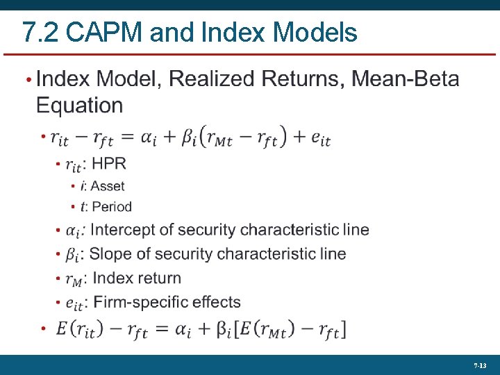
7. 2 CAPM and Index Models 7 -13

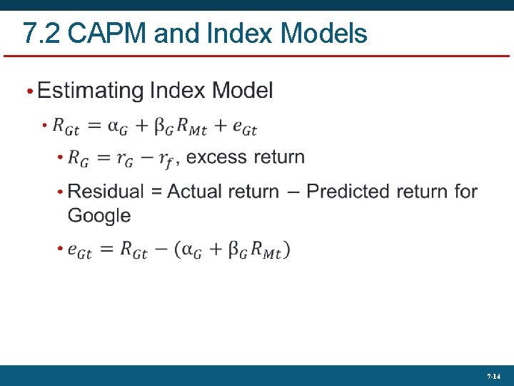
7. 2 CAPM and Index Models • 7 -14

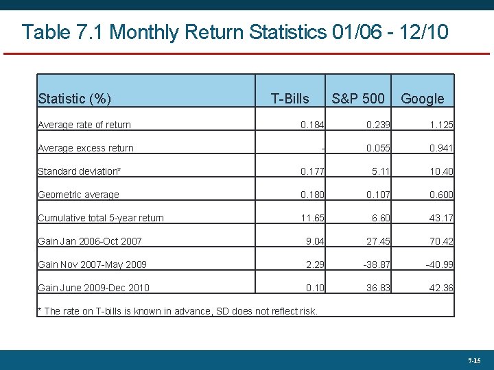
Table 7. 1 Monthly Return Statistics 01/06 - 12/10 Statistic (%) T-Bills S&P 500 Google Average rate of return 0. 184 0. 239 1. 125 Average excess return - 0. 055 0. 941 Standard deviation* 0. 177 5. 11 10. 40 Geometric average 0. 180 0. 107 0. 600 Cumulative total 5 -year return 11. 65 6. 60 43. 17 Gain Jan 2006 -Oct 2007 9. 04 27. 45 70. 42 Gain Nov 2007 -May 2009 2. 29 -38. 87 -40. 99 Gain June 2009 -Dec 2010 0. 10 36. 83 42. 36 * The rate on T-bills is known in advance, SD does not reflect risk. 7 -15

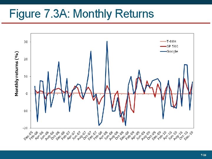
Figure 7. 3 A: Monthly Returns 7 -16

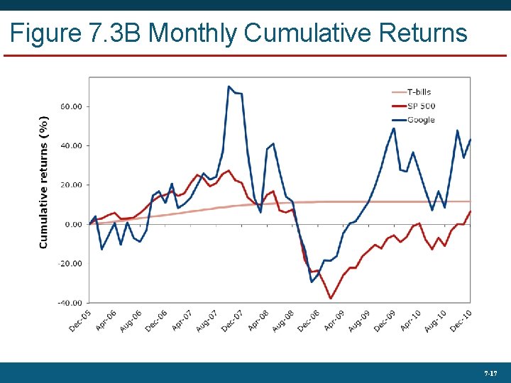
Figure 7. 3 B Monthly Cumulative Returns 7 -17

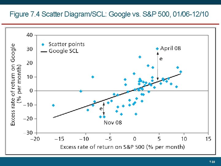
Figure 7. 4 Scatter Diagram/SCL: Google vs. S&P 500, 01/06 -12/10 7 -18

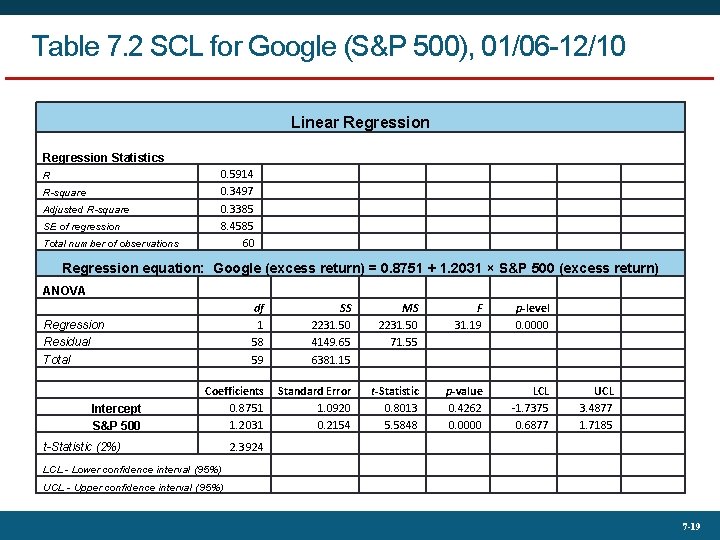
Table 7. 2 SCL for Google (S&P 500), 01/06 -12/10 Linear Regression Statistics R R-square Adjusted R-square SE of regression Total number of observations 0. 5914 0. 3497 0. 3385 8. 4585 60 Regression equation: Google (excess return) = 0. 8751 + 1. 2031 × S&P 500 (excess return) ANOVA df 1 58 59 SS 2231. 50 4149. 65 6381. 15 MS 2231. 50 71. 55 F 31. 19 p-level 0. 0000 Coefficients 0. 8751 1. 2031 Standard Error 1. 0920 0. 2154 t-Statistic 0. 8013 5. 5848 p-value 0. 4262 0. 0000 LCL -1. 7375 0. 6877 Regression Residual Total Intercept S&P 500 t-Statistic (2%) UCL 3. 4877 1. 7185 2. 3924 LCL - Lower confidence interval (95%) UCL - Upper confidence interval (95%) 7 -19

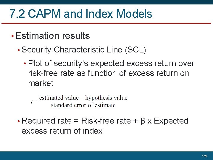
7. 2 CAPM and Index Models • Estimation results • Security Characteristic Line (SCL) • Plot of security’s expected excess return over risk-free rate as function of excess return on market • Required rate = Risk-free rate + β x Expected excess return of index 7 -20

7. 2 CAPM and Index Models • Predicting Betas • Mean reversion • Betas move towards mean over time • To predict future betas, adjust estimates from historical data to account for regression towards 1. 0 7 -21

7. 3 CAPM and the Real World • CAPM is false based on validity of its assumptions • Useful predictor of expected returns • Untestable as a theory • Principles still valid • Investors should diversify • Systematic risk is the risk that matters • Well-diversified risky portfolio can be suitable for wide range of investors 7 -22

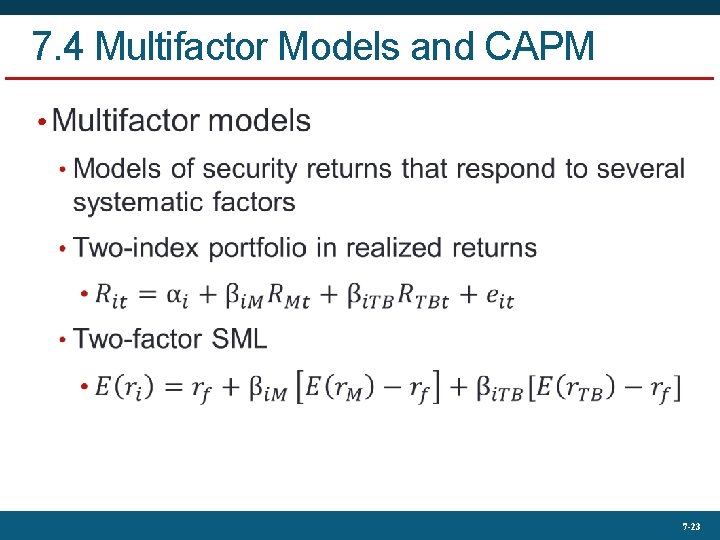
7. 4 Multifactor Models and CAPM • 7 -23

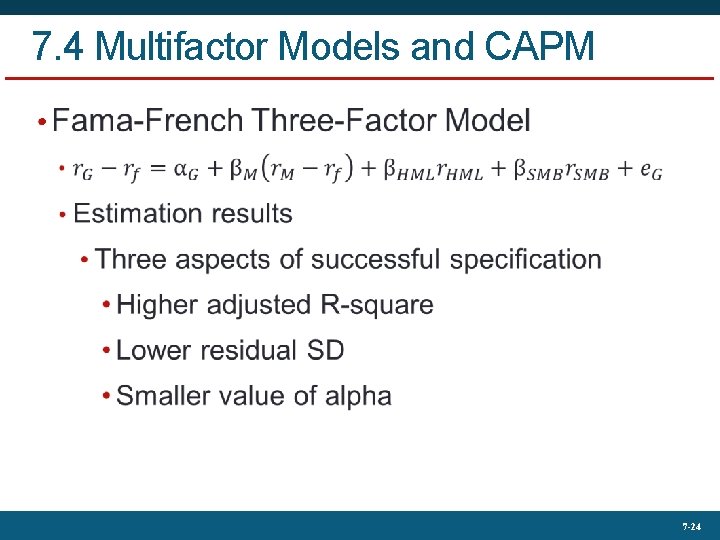
7. 4 Multifactor Models and CAPM • 7 -24

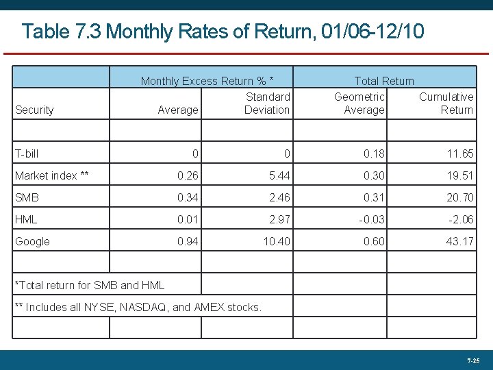
Table 7. 3 Monthly Rates of Return, 01/06 -12/10 Security Monthly Excess Return % * Standard Average Deviation T-bill Total Return Geometric Cumulative Average Return 0 0 0. 18 11. 65 Market index ** 0. 26 5. 44 0. 30 19. 51 SMB 0. 34 2. 46 0. 31 20. 70 HML 0. 01 2. 97 -0. 03 -2. 06 Google 0. 94 10. 40 0. 60 43. 17 *Total return for SMB and HML ** Includes all NYSE, NASDAQ, and AMEX stocks. 7 -25

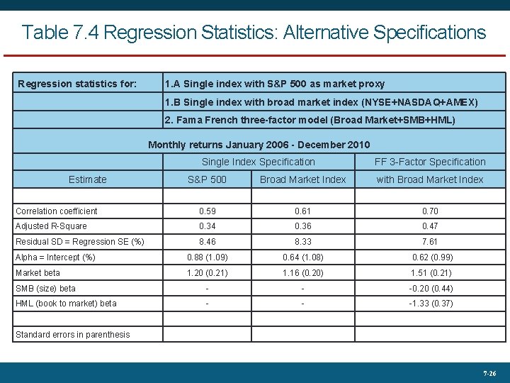
Table 7. 4 Regression Statistics: Alternative Specifications Regression statistics for: 1. A Single index with S&P 500 as market proxy 1. B Single index with broad market index (NYSE+NASDAQ+AMEX) 2. Fama French three-factor model (Broad Market+SMB+HML) Monthly returns January 2006 - December 2010 Single Index Specification Estimate FF 3 -Factor Specification S&P 500 Broad Market Index with Broad Market Index Correlation coefficient 0. 59 0. 61 0. 70 Adjusted R-Square 0. 34 0. 36 0. 47 Residual SD = Regression SE (%) 8. 46 8. 33 7. 61 Alpha = Intercept (%) 0. 88 (1. 09) 0. 64 (1. 08) 0. 62 (0. 99) Market beta 1. 20 (0. 21) 1. 16 (0. 20) 1. 51 (0. 21) SMB (size) beta - - -0. 20 (0. 44) HML (book to market) beta - - -1. 33 (0. 37) Standard errors in parenthesis 7 -26

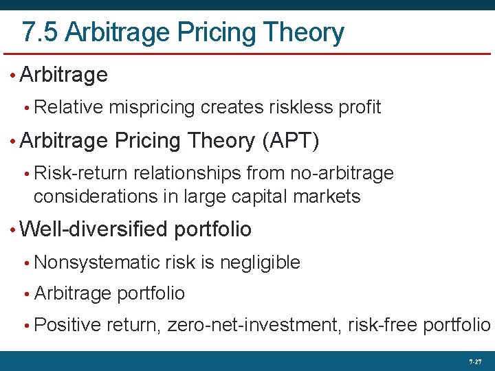
7. 5 Arbitrage Pricing Theory • Arbitrage • Relative mispricing creates riskless profit • Arbitrage Pricing Theory (APT) • Risk-return relationships from no-arbitrage considerations in large capital markets • Well-diversified portfolio • Nonsystematic risk is negligible • Arbitrage portfolio • Positive return, zero-net-investment, risk-free portfolio 7 -27

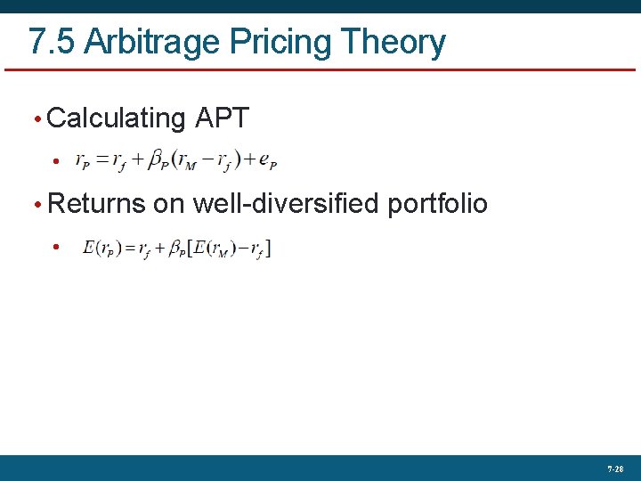
7. 5 Arbitrage Pricing Theory • Calculating APT • • Returns on well-diversified portfolio • 7 -28

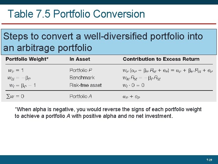
Table 7. 5 Portfolio Conversion Steps to convert a well-diversified portfolio into an arbitrage portfolio *When alpha is negative, you would reverse the signs of each portfolio weight to achieve a portfolio A with positive alpha and no net investment. 7 -29

Table 7. 6 Largest Capitalization Stocks in S&P 500 Stock Weight 7 -30

Table 7. 7 Regression Statistics of S&P 500 Portfolio on Benchmark Portfolio, 01/06 -12/10 Linear Regression Statistics R 0. 9933 R-square 0. 9866 Adjusted R-square 0. 9864 Annualized Regression SE 0. 5968 2. 067 Total number of observations 60 S&P 500 = - 0. 1909 + 0. 9337 × Benchmark Standard Coefficients Error t-stat p-level Intercept -0. 1909 0. 0771 -2. 4752 0. 0163 Benchmark 0. 9337 0. 0143 65. 3434 0. 0000 7 -31

Table 7. 8 Annual Standard Deviation Period Real Rate Inflation Rate Nominal Rate 1/1 /06 - 12/31/10 1. 46 0. 61 1/1/96 - 12/31/00 0. 57 0. 54 0. 17 1/1/86 - 12/31/90 0. 86 0. 83 0. 37 7 -32

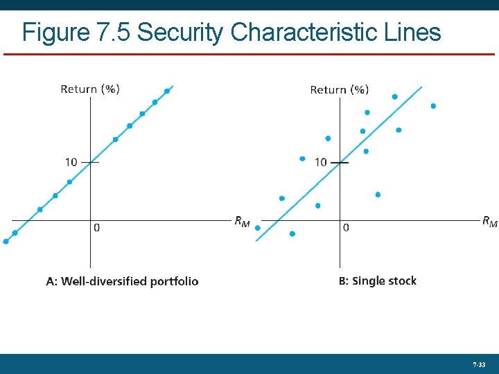
Figure 7. 5 Security Characteristic Lines 7 -33

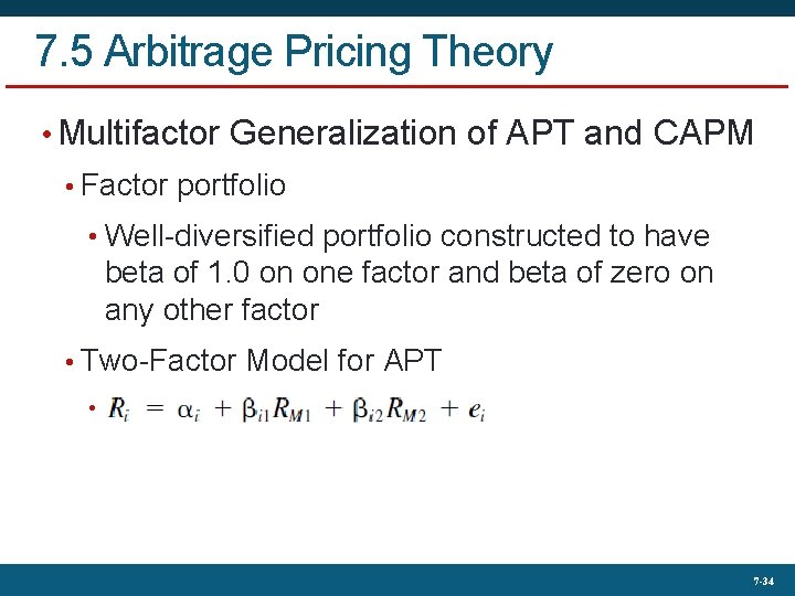
7. 5 Arbitrage Pricing Theory • Multifactor Generalization of APT and CAPM • Factor portfolio • Well-diversified portfolio constructed to have beta of 1. 0 on one factor and beta of zero on any other factor • Two-Factor Model for APT • 7 -34

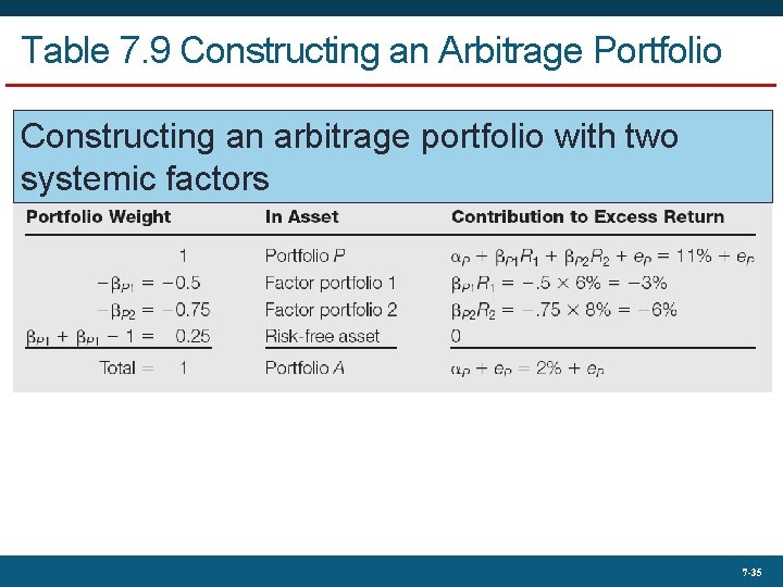
Table 7. 9 Constructing an Arbitrage Portfolio Constructing an arbitrage portfolio with two systemic factors 7 -35