CAPE in Tropical Cyclones John Molinari David Romps

CAPE in Tropical Cyclones John Molinari, David Romps, David Vollaro, and Leon Nguyen

• Description of data • Calculation of CAPE • Upshear-downshear differences in CAPE in tropical cyclones • Vertical distribution of buoyancy

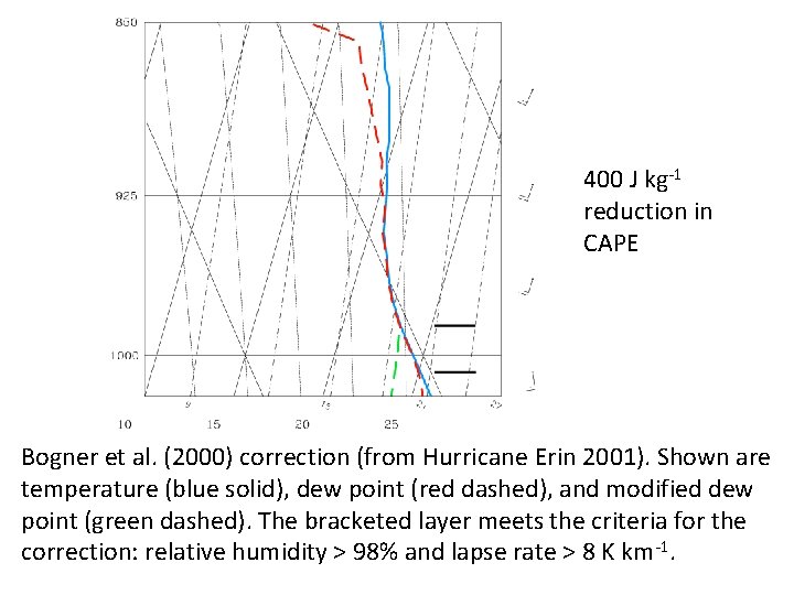
G-IV soundings Processed by Sim Aberson using Editsonde 32 storms over 7 years (1997 -1999; 2002 -2005) 3% in tropical depressions, 24% in tropical storms, remainder in hurricanes of all intensities Any data listed as questionable by Editsonde was removed, including the first 30 s after sonde release (about 600 m) One additional correction for rh < 10% just above the surface (only 6 sondes) Bogner et al. (2000) correction for near dry-adiabatic saturated layers below cloud base (3. 3% of sondes)

400 J kg-1 reduction in CAPE Bogner et al. (2000) correction (from Hurricane Erin 2001). Shown are temperature (blue solid), dew point (red dashed), and modified dew point (green dashed). The bracketed layer meets the criteria for the correction: relative humidity > 98% and lapse rate > 8 K km-1.

Sonde data interpolated to 100 m levels Linear interpolation of T and Td across gaps of no more than 400 m. No CAPE computed for larger gaps Sondes used only within 1000 km of the tropical cyclone center Release point had to be above the 400 h. Pa level 2458 sondes left for analysis Above sonde release level, append lapse rate interpolated from the nearest (in time) ECMWF operational analysis interpolated to the sonde point

Bogner et al. (2000): used omega dropwindsondes released at an average pressure of 450 h. Pa; appended mean tropical cyclone sounding above Two thirds of pseudoadiabatic CAPE was above the mean release level of the sondes G-IV sondes in this study have an average release level of 13. 06 km (near 180 h. Pa), standard deviation 0. 59 km. Thus most of the tropopause is directly measured by the sonde, a major benefit for CAPE calculations

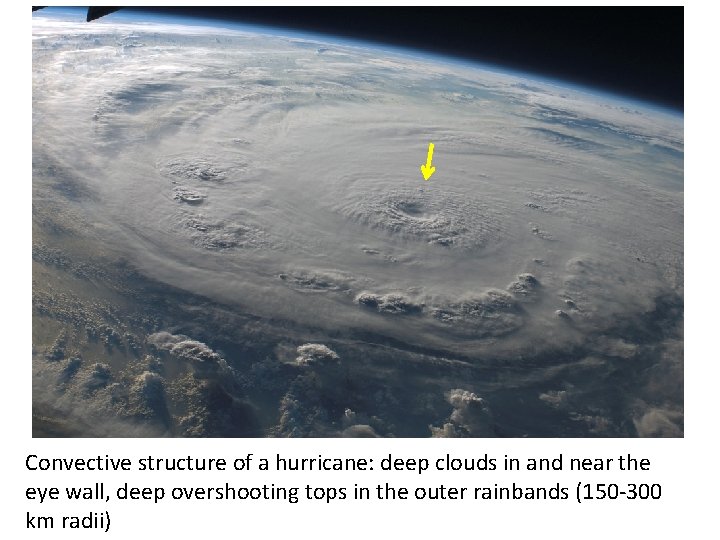
Convective structure of a hurricane: deep clouds in and near the eye wall, deep overshooting tops in the outer rainbands (150 -300 km radii)

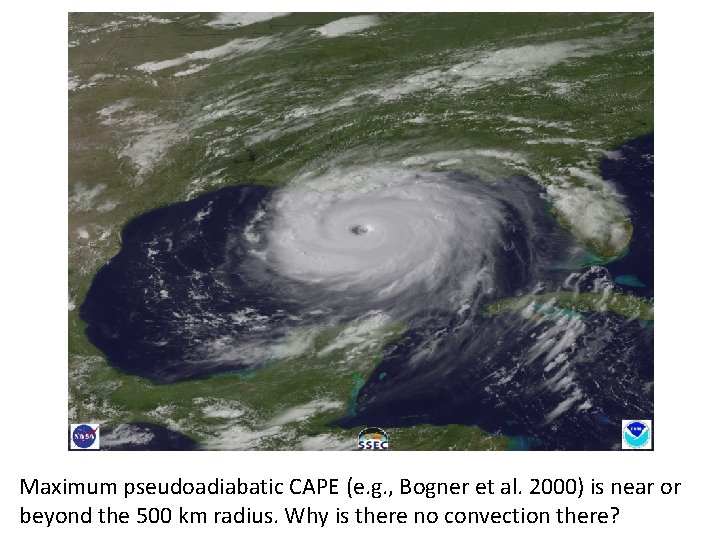
Maximum pseudoadiabatic CAPE (e. g. , Bogner et al. 2000) is near or beyond the 500 km radius. Why is there no convection there?

Pseudoadiabatic CAPE: condensate falls immediately, no condensate loading, no mixing with environment. This is used most commonly. Reversible CAPE: No mixing with the environment, but keep all condensate with the parcel. Xu and Emanuel (1989) argued that the tropics were near moist neutral for reversible CAPE Romps and Kuang 2010: calculate parcel properties in deep convection in the tropics, including condensate loading, entrainment, and heating by fusion, using a detailed parcel model CAPE can be calculated from these results by calculating buoyancy that includes all these effects

How important is fusion heating in updrafts? Zipser (2003), Romps and Kuang (2010), and Fierro et al. (2012): observations and models both show that fusion heating is required for updrafts to reach the tropopause in the tropics. Undilute ascent does not occur! Williams and Renno (1993): increase in CAPE from fusion heating almost exactly offsets the decrease in CAPE from condensate loading. Thus reversible CAPE with fusion approximately equals pseudoadiabatic CAPE without fusion In this study, water is assumed to transition linearly to ice between temperatures of 273. 15 and 240 K

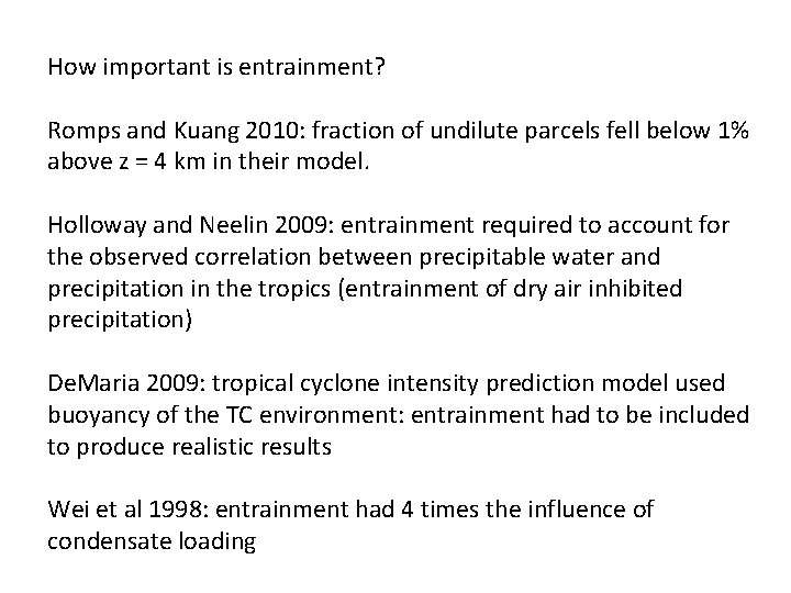
How important is entrainment? Romps and Kuang 2010: fraction of undilute parcels fell below 1% above z = 4 km in their model. Holloway and Neelin 2009: entrainment required to account for the observed correlation between precipitable water and precipitation in the tropics (entrainment of dry air inhibited precipitation) De. Maria 2009: tropical cyclone intensity prediction model used buoyancy of the TC environment: entrainment had to be included to produce realistic results Wei et al 1998: entrainment had 4 times the influence of condensate loading

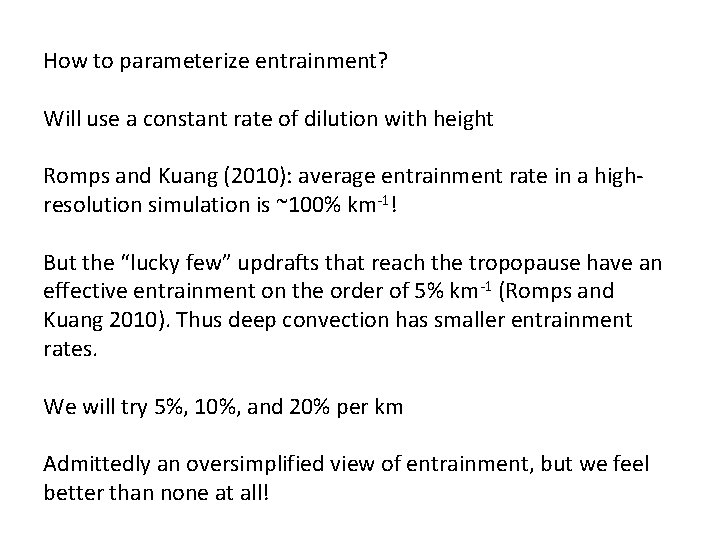
How to parameterize entrainment? Will use a constant rate of dilution with height Romps and Kuang (2010): average entrainment rate in a highresolution simulation is ~100% km-1! But the “lucky few” updrafts that reach the tropopause have an effective entrainment on the order of 5% km-1 (Romps and Kuang 2010). Thus deep convection has smaller entrainment rates. We will try 5%, 10%, and 20% per km Admittedly an oversimplified view of entrainment, but we feel better than none at all!

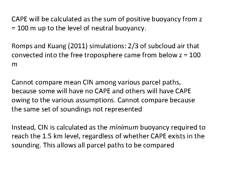
CAPE will be calculated as the sum of positive buoyancy from z = 100 m up to the level of neutral buoyancy. Romps and Kuang (2011) simulations: 2/3 of subcloud air that convected into the free troposphere came from below z = 100 m Cannot compare mean CIN among various parcel paths, because some will have no CAPE and others will have CAPE owing to the various assumptions. Cannot compare because the same set of soundings not represented Instead, CIN is calculated as the minimum buoyancy required to reach the 1. 5 km level, regardless of whether CAPE exists in the sounding. This allows all parcel paths to be compared

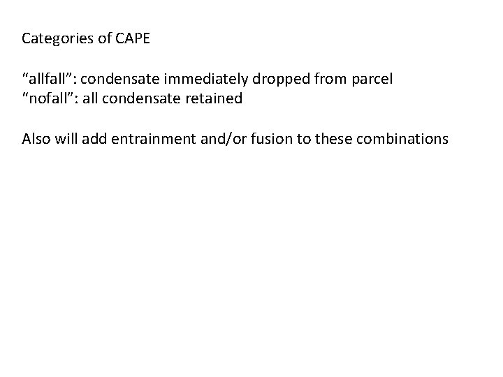
Categories of CAPE “allfall”: condensate immediately dropped from parcel “nofall”: all condensate retained Also will add entrainment and/or fusion to these combinations

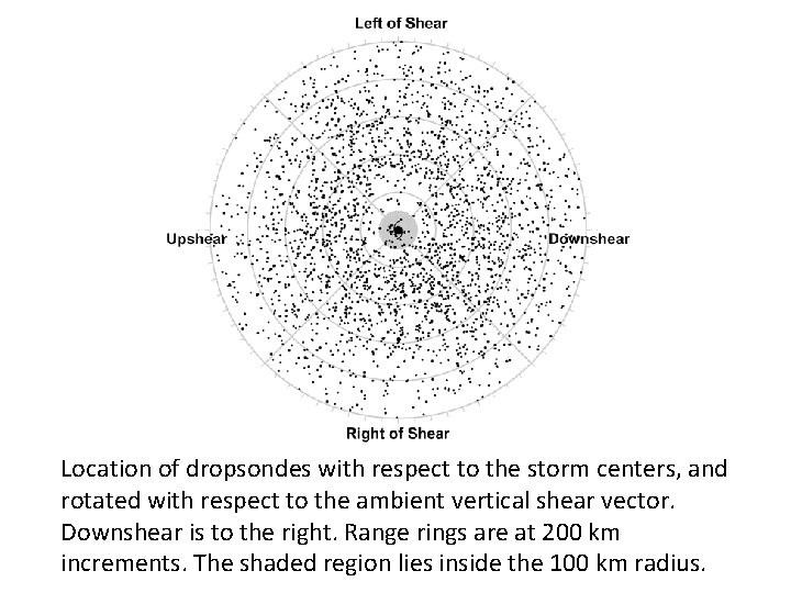
Location of dropsondes with respect to the storm centers, and rotated with respect to the ambient vertical shear vector. Downshear is to the right. Range rings are at 200 km increments. The shaded region lies inside the 100 km radius.

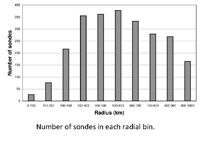
Number of sondes in each radial bin.

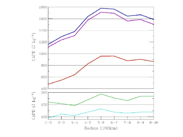
CAPE (J kg-1) vs radius determined by averaging from the dropsondes over 100 -km radial bins. Five different parcel paths are shown: Blue: pseudoadiabatic; Red: traditional reversible; Purple: reversible with fusion; Green: allfall, entrainment = 10% km-1, with fusion; Cyan: nofall, entrainment = 10% km-1, no fusion.

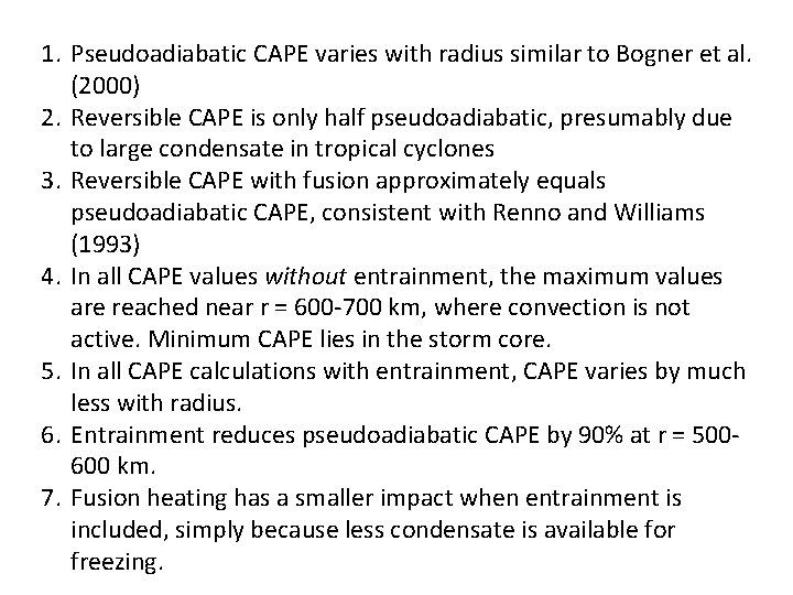
1. Pseudoadiabatic CAPE varies with radius similar to Bogner et al. (2000) 2. Reversible CAPE is only half pseudoadiabatic, presumably due to large condensate in tropical cyclones 3. Reversible CAPE with fusion approximately equals pseudoadiabatic CAPE, consistent with Renno and Williams (1993) 4. In all CAPE values without entrainment, the maximum values are reached near r = 600 -700 km, where convection is not active. Minimum CAPE lies in the storm core. 5. In all CAPE calculations with entrainment, CAPE varies by much less with radius. 6. Entrainment reduces pseudoadiabatic CAPE by 90% at r = 500600 km. 7. Fusion heating has a smaller impact when entrainment is included, simply because less condensate is available for freezing.

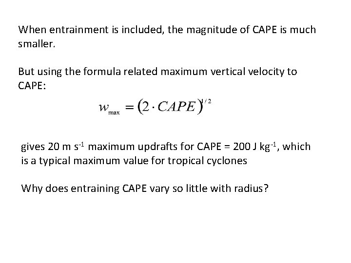
When entrainment is included, the magnitude of CAPE is much smaller. But using the formula related maximum vertical velocity to CAPE: gives 20 m s-1 maximum updrafts for CAPE = 200 J kg-1, which is a typical maximum value for tropical cyclones Why does entraining CAPE vary so little with radius?

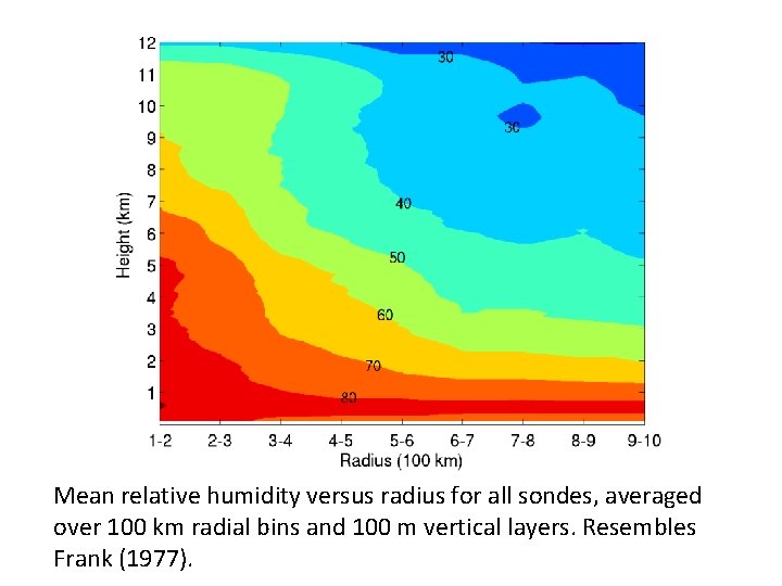
Mean relative humidity versus radius for all sondes, averaged over 100 km radial bins and 100 m vertical layers. Resembles Frank (1977).

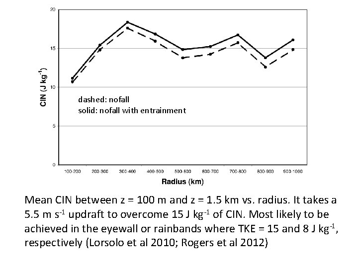
dashed: nofall solid: nofall with entrainment Mean CIN between z = 100 m and z = 1. 5 km vs. radius. It takes a 5. 5 m s-1 updraft to overcome 15 J kg-1 of CIN. Most likely to be achieved in the eyewall or rainbands where TKE = 15 and 8 J kg-1, respectively (Lorsolo et al 2010; Rogers et al 2012)

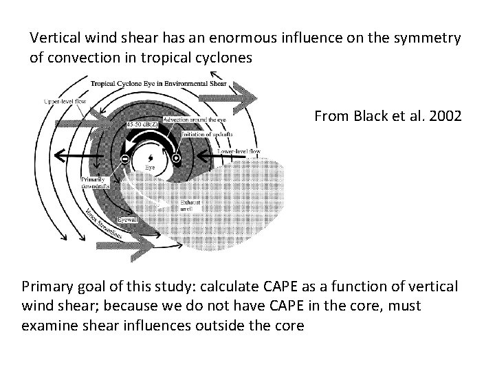
Vertical wind shear has an enormous influence on the symmetry of convection in tropical cyclones From Black et al. 2002 Primary goal of this study: calculate CAPE as a function of vertical wind shear; because we do not have CAPE in the core, must examine shear influences outside the core

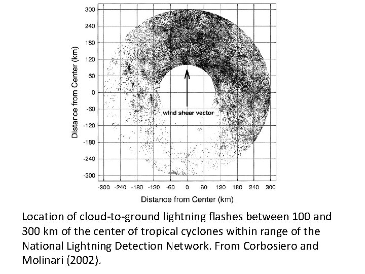
Location of cloud-to-ground lightning flashes between 100 and 300 km of the center of tropical cyclones within range of the National Lightning Detection Network. From Corbosiero and Molinari (2002).

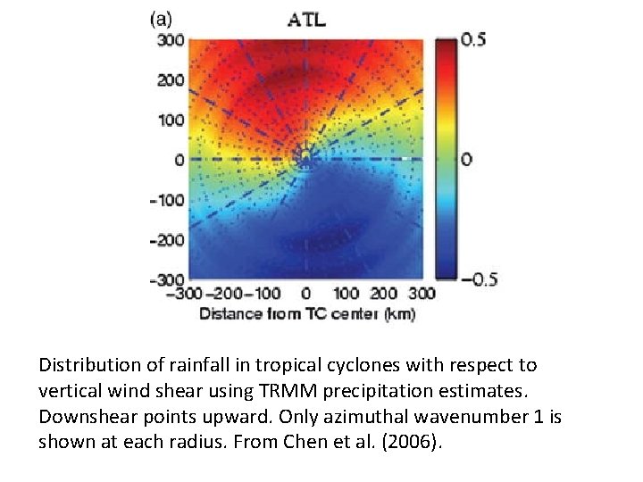
Distribution of rainfall in tropical cyclones with respect to vertical wind shear using TRMM precipitation estimates. Downshear points upward. Only azimuthal wavenumber 1 is shown at each radius. From Chen et al. (2006).

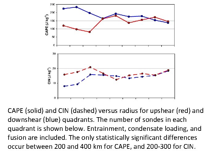
CAPE (solid) and CIN (dashed) versus radius for upshear (red) and downshear (blue) quadrants. The number of sondes in each quadrant is shown below. Entrainment, condensate loading, and fusion are included. The only statistically significant differences occur between 200 and 400 km for CAPE, and 200 -300 for CIN.

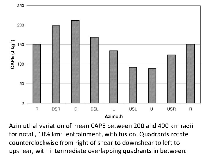
Azimuthal variation of mean CAPE between 200 and 400 km radii for nofall, 10% km-1 entrainment, with fusion. Quadrants rotate counterclockwise from right of shear to downshear to left to upshear, with intermediate overlapping quadrants in between.

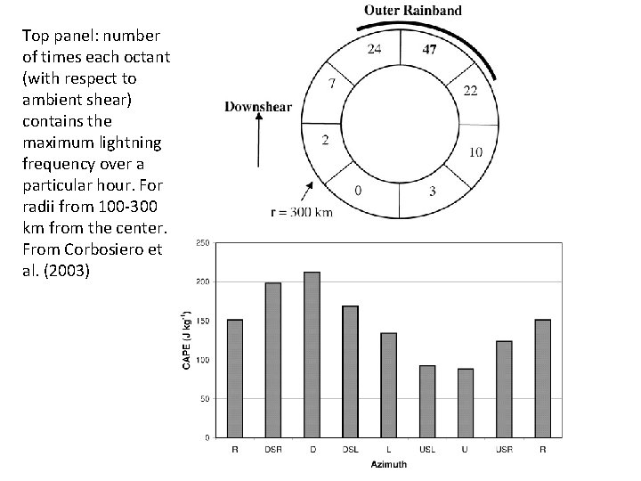
Top panel: number of times each octant (with respect to ambient shear) contains the maximum lightning frequency over a particular hour. For radii from 100 -300 km from the center. From Corbosiero et al. (2003)

Conclusion from the previous 3 figures: the most lightning (i. e. , the strongest and/or most frequent convection) occurs where there is the most CAPE: in the inner core, not at radii of 600700 km; and downshear, not upshear. It is not correct to argue that CAPE must be smallest where convection is most frequent The inclusion of entrainment is necessary to obtain this result Why does entrainment contribute to upshear-downshear differences?

∆T ∆rh Vertical distribution of temperature (Units: 0. 1 K) and relative humidity (%) differences, downshear quadrant – upshear quadrant, for r = 200 -400 km.

The larger CAPE downshear than upshear arises from • Lower midtropospheric temperatures producing greater parcel buoyancy • Larger surface humidity producing greater parcel buoyancy, and • Much larger free troposphere relative humidity reducing the impact of entrainment on buoyancy The first two most likely arise from stronger upward motion downshear. The last appears to occur due to 16% larger surface wind speed downshear (not shown).

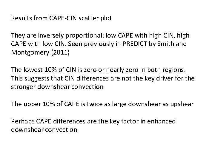
One benefit of G-IV sondes: their large number allows the upper 10% of CAPE and lower 10% CIN to be measured. Outside the 100 km radius, fractional coverage of deep convection is 10% or less (even true in core). Thus the 90 th percentile might be relevant to examine

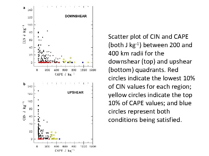
Scatter plot of CIN and CAPE (both J kg-1) between 200 and 400 km radii for the downshear (top) and upshear (bottom) quadrants. Red circles indicate the lowest 10% of CIN values for each region; yellow circles indicate the top 10% of CAPE values; and blue circles represent both conditions being satisfied.

Results from CAPE-CIN scatter plot They are inversely proportional: low CAPE with high CIN, high CAPE with low CIN. Seen previously in PREDICT by Smith and Montgomery (2011) The lowest 10% of CIN is zero or nearly zero in both regions. This suggests that CIN differences are not the key driver for the stronger downshear convection The upper 10% of CAPE is twice as large downshear as upshear Perhaps CAPE differences are the key factor in enhanced downshear convection

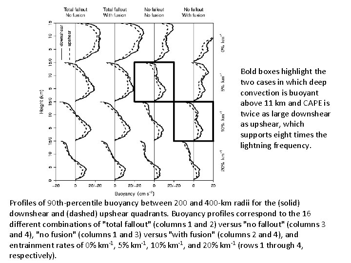
Next consider all combinations of with and without fusion, with and without condensate loading, and for entrainment values of 0, 5, 10, and 20% km-1. How do the vertical profiles of buoyancy vary? How do we choose which is best? Because downshear CAPE is 6 X upshear CAPE (Corbosiero and Molinari 2002, 2003), we ask that the 90 th percentile of downshear CAPE be twice that upshear. Because lightning frequency is proportional to w 6 (Baker et al. 1999) and thus CAPE 3, twice the CAPE gives 8 X the lightning frequency, close to observed. Also require that downshear parcels reach the top third of the troposphere (LNB at or above 11 km), while upshear do not.

Bold boxes highlight the two cases in which deep convection is buoyant above 11 km and CAPE is twice as large downshear as upshear, which supports eight times the lightning frequency. Profiles of 90 th-percentile buoyancy between 200 and 400 -km radii for the (solid) downshear and (dashed) upshear quadrants. Buoyancy profiles correspond to the 16 different combinations of "total fallout" (columns 1 and 2) versus "no fallout" (columns 3 and 4), "no fusion" (columns 1 and 3) versus "with fusion" (columns 2 and 4), and entrainment rates of 0% km-1, 5% km-1, 10% km-1, and 20% km-1 (rows 1 through 4, respectively).

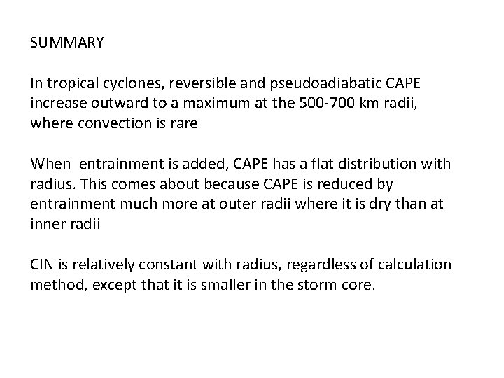
SUMMARY In tropical cyclones, reversible and pseudoadiabatic CAPE increase outward to a maximum at the 500 -700 km radii, where convection is rare When entrainment is added, CAPE has a flat distribution with radius. This comes about because CAPE is reduced by entrainment much more at outer radii where it is dry than at inner radii CIN is relatively constant with radius, regardless of calculation method, except that it is smaller in the storm core.

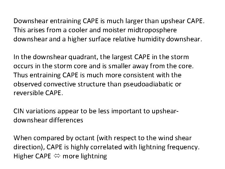
Downshear entraining CAPE is much larger than upshear CAPE. This arises from a cooler and moister midtroposphere downshear and a higher surface relative humidity downshear. In the downshear quadrant, the largest CAPE in the storm occurs in the storm core and is smaller away from the core. Thus entraining CAPE is much more consistent with the observed convective structure than pseudoadiabatic or reversible CAPE. CIN variations appear to be less important to upsheardownshear differences When compared by octant (with respect to the wind shear direction), CAPE is highly correlated with lightning frequency. Higher CAPE more lightning

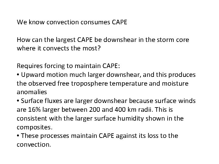
We know convection consumes CAPE How can the largest CAPE be downshear in the storm core where it convects the most? Requires forcing to maintain CAPE: • Upward motion much larger downshear, and this produces the observed free troposphere temperature and moisture anomalies • Surface fluxes are larger downshear because surface winds are 16% larger between 200 and 400 km radii. This is consistent with the larger surface humidity shown in the composites. • These processes maintain CAPE against its loss to the convection.

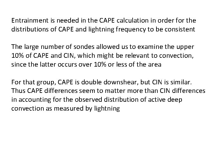
Entrainment is needed in the CAPE calculation in order for the distributions of CAPE and lightning frequency to be consistent The large number of sondes allowed us to examine the upper 10% of CAPE and CIN, which might be relevant to convection, since the latter occurs over 10% or less of the area For that group, CAPE is double downshear, but CIN is similar. Thus CAPE differences seem to matter more than CIN differences in accounting for the observed distribution of active deep convection as measured by lightning

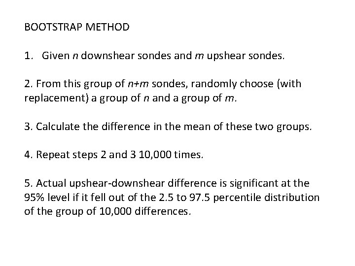
BOOTSTRAP METHOD 1. Given n downshear sondes and m upshear sondes. 2. From this group of n+m sondes, randomly choose (with replacement) a group of n and a group of m. 3. Calculate the difference in the mean of these two groups. 4. Repeat steps 2 and 3 10, 000 times. 5. Actual upshear-downshear difference is significant at the 95% level if it fell out of the 2. 5 to 97. 5 percentile distribution of the group of 10, 000 differences.

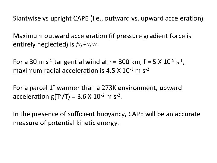
Slantwise vs upright CAPE (i. e. , outward vs. upward acceleration) Maximum outward acceleration (if pressure gradient force is entirely neglected) is fvλ + vλ 2/r For a 30 m s-1 tangential wind at r = 300 km, f = 5 X 10 -5 s-1, maximum radial acceleration is 4. 5 X 10 -3 m s-2 For a parcel 1˚ warmer than a 273 K environment, upward acceleration g(T’/T) = 3. 6 X 10 -2 m s-2. In the presence of sufficient buoyancy, CAPE will be an accurate measure of potential kinetic energy.