Candidate Zones Z Tessellated study area Want zones

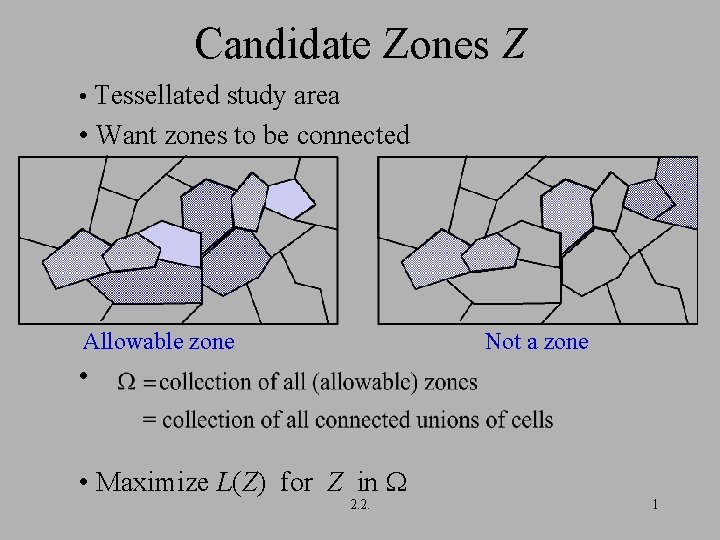
Candidate Zones Z • Tessellated study area • Want zones to be connected Allowable zone Not a zone • • Maximize L(Z) for Z in 2. 2. 1

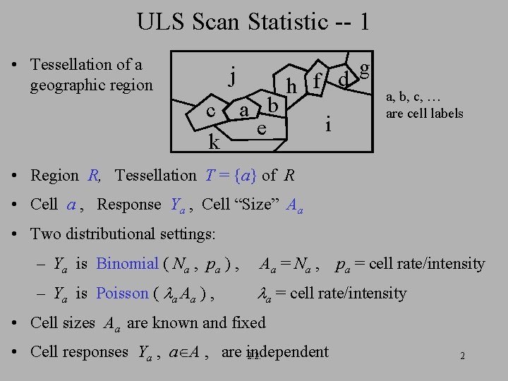
ULS Scan Statistic -- 1 • Tessellation of a geographic region j c a b e k h f d i g a, b, c, … are cell labels • Region R, Tessellation T = {a} of R • Cell a , Response Ya , Cell “Size” Aa • Two distributional settings: – Ya is Binomial ( Na , pa ) , Aa = Na , – Ya is Poisson ( a Aa ) , a = cell rate/intensity pa = cell rate/intensity • Cell sizes Aa are known and fixed • Cell responses Ya , a A , are independent 2. 2. 2

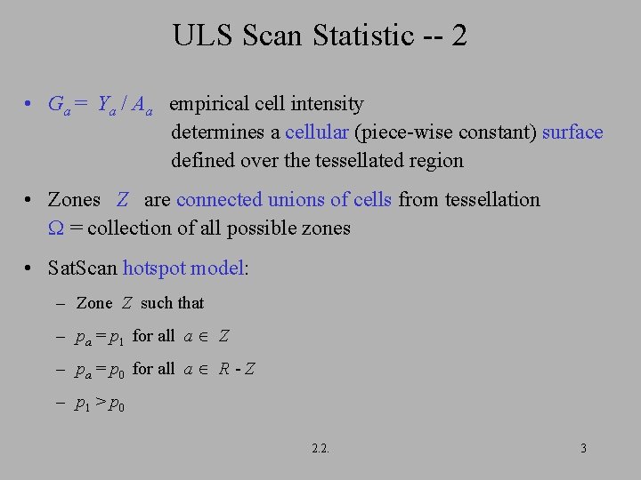
ULS Scan Statistic -- 2 • Ga = Ya / Aa empirical cell intensity determines a cellular (piece-wise constant) surface defined over the tessellated region • Zones Z are connected unions of cells from tessellation = collection of all possible zones • Sat. Scan hotspot model: – Zone Z such that – pa = p 1 for all a Z – pa = p 0 for all a R - Z – p 1 > p 0 2. 2. 3

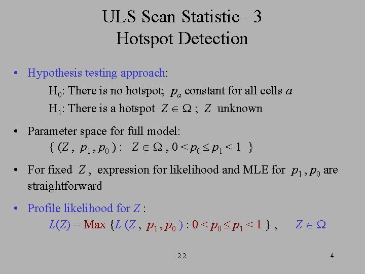
ULS Scan Statistic– 3 Hotspot Detection • Hypothesis testing approach: H 0: There is no hotspot; pa constant for all cells a H 1: There is a hotspot Z ; Z unknown • Parameter space for full model: { (Z , p 1 , p 0 ) : Z , 0 < p 0 p 1 < 1 } • For fixed Z , expression for likelihood and MLE for p 1 , p 0 are straightforward • Profile likelihood for Z : L(Z) = Max {L (Z , p 1 , p 0 ) : 0 < p 0 p 1 < 1 } , 2. 2. Z 4

ULS Scan Statistic– 4 Hotspot Estimation • is finite but large • Maximizing L(Z) , Z , by exhaustive search impractical • Possible optimization methods: – Stochastic optimization (annealing, GA, etc. ) – Reduction of to 0 with 0 and 0 small enough for exhaustive search • Possible reductions of to 0 : – Expanding circles An a priori reduction which depends only on the tessellation and not on the data – Upper level sets of empirical intensity surface (Tree-Structured SATScan) An adaptive, data-dependent, reduction allowing flexible shapes for zones in 0. Data dependence must be incorporated into simulations. 5 2. 2.

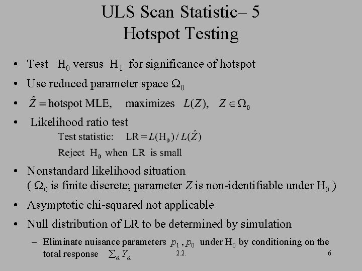
ULS Scan Statistic– 5 Hotspot Testing • Test H 0 versus H 1 for significance of hotspot • Use reduced parameter space 0 • • Likelihood ratio test • Nonstandard likelihood situation ( 0 is finite discrete; parameter Z is non-identifiable under H 0 ) • Asymptotic chi-squared not applicable • Null distribution of LR to be determined by simulation – Eliminate nuisance parameters p 1 , p 0 under H 0 by conditioning on the 2. 2. 6 total response a Ya

ULS Scan Statistic– 6 • Goal: Identify geographic zone(s) in which a response is significantly elevated relative to the rest of a region • A list of candidate zones Z is specified a priori. – This list becomes part of the parameter space and the zone must be estimated from within this list. – Each candidate zone should generally be spatially connected, e. g. , a union of contiguous spatial units or cells. – Longer lists of candidate zones are usually preferable – Expanding circles or ellipses about specified centers are a common method of generating the list 2. 2. 7

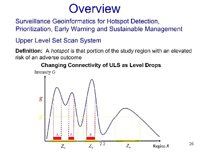
ULS Scan Statistic– 7 • Question: Are there data-driven (rather than a priori) ways of selecting the list of candidate zones ? • Motivation for the question: A human being can look at a map and quickly determine a reasonable set of candidate zones and eliminate many other zones as obviously uninteresting. Can the computer do the same thing? • A data-driven proposal: Candidate zones are the connected components of the upper level sets of the response surface. The candidate zones have a tree structure, which may assist in automated detection of multiple, but geographically separate, elevated zones. • Null distribution: If the list is data-driven (i. e. , random), its variability must be accounted for in the null distribution. A new list must be developed for 2. 2. each simulated data set. 8

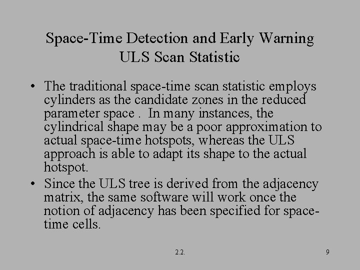
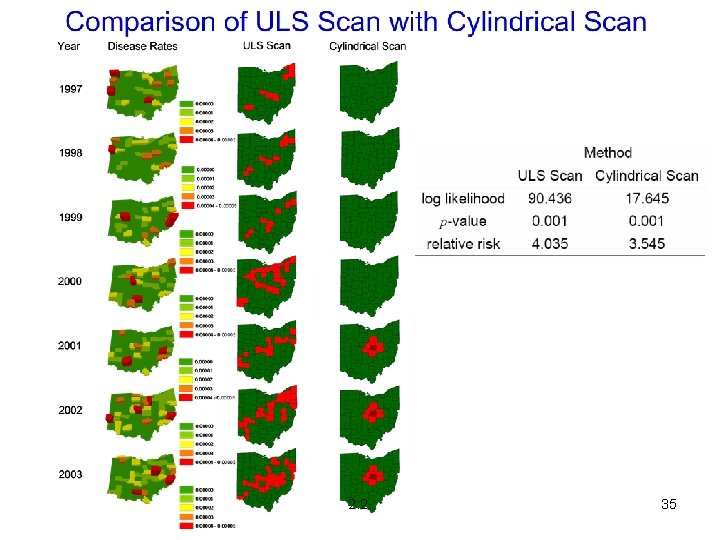
Space-Time Detection and Early Warning ULS Scan Statistic • The traditional space-time scan statistic employs cylinders as the candidate zones in the reduced parameter space. In many instances, the cylindrical shape may be a poor approximation to actual space-time hotspots, whereas the ULS approach is able to adapt its shape to the actual hotspot. • Since the ULS tree is derived from the adjacency matrix, the same software will work once the notion of adjacency has been specified for spacetime cells. 2. 2. 9

Hotspot Detection for Continuous Responses • Human Health Context: Ø Blood pressure levels for spatial variation in hypertension Ø Cancer survival (censoring issues) • Environmental Context: Ø Landscape metrics such as forest cover, fragmentation, etc. Ø Pollutant loadings Ø Animal abundance 2. 2. 10

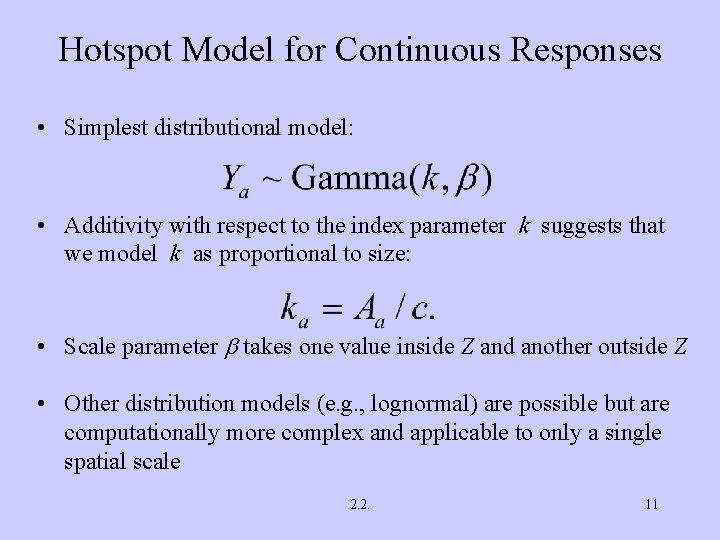
Hotspot Model for Continuous Responses • Simplest distributional model: • Additivity with respect to the index parameter k suggests that we model k as proportional to size: • Scale parameter takes one value inside Z and another outside Z • Other distribution models (e. g. , lognormal) are possible but are computationally more complex and applicable to only a single spatial scale 2. 2. 11

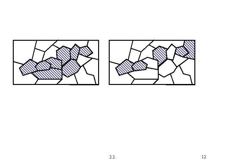
2. 2. 12

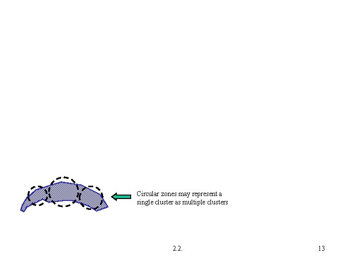
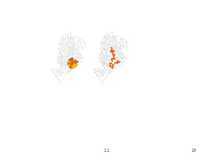
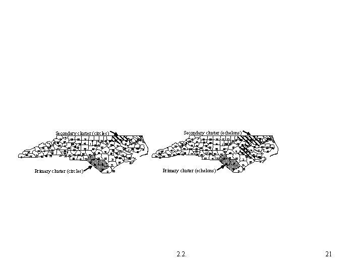
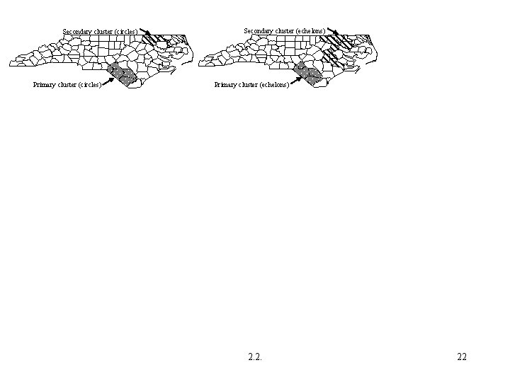
Circular zones may represent a single cluster as multiple clusters 2. 2. 13

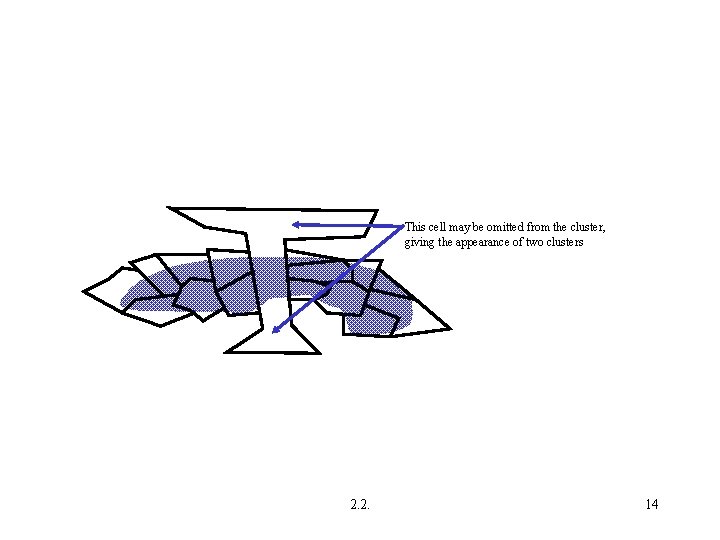
This cell may be omitted from the cluster, giving the appearance of two clusters 2. 2. 14

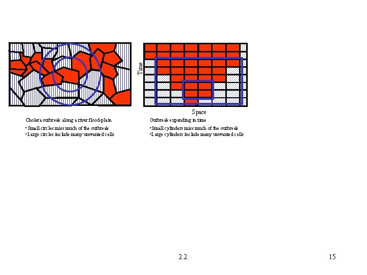
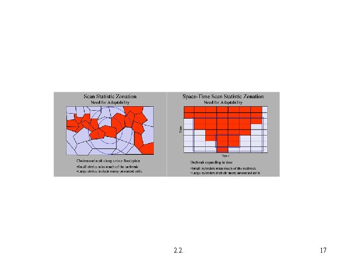
Time Space Cholera outbreak along a river flood-plain Outbreak expanding in time • Small circles miss much of the outbreak • Large circles include many unwanted cells • Small cylinders miss much of the outbreak • Large cylinders include many unwanted cells 2. 2. 15

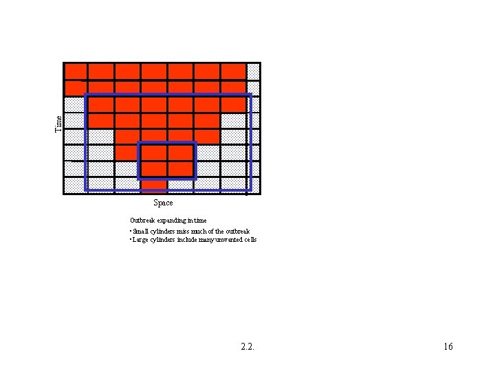
Time Space Outbreak expanding in time • Small cylinders miss much of the outbreak • Large cylinders include many unwanted cells 2. 2. 16

2. 2. 17

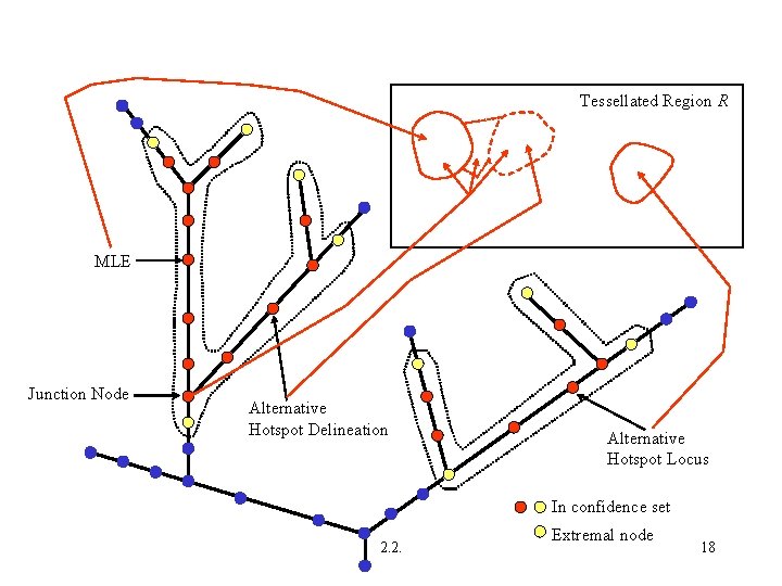
Tessellated Region R MLE Junction Node Alternative Hotspot Delineation Alternative Hotspot Locus In confidence set 2. 2. Extremal node 18

2. 2. 19

2. 2. 20

Secondary cluster (echelons) Secondary cluster (circles) 2 87 38 57 5 3 86 85 79 17 73 39 91 6 95 97 35 99 34 41 1 68 32 14 2 61 3 0 2 9 92 1 00 4 9 58 1 2 7 6 1 9 8 0 56 18 44 11 81 55 53 43 51 23 36 60 13 84 62 63 0 88 45 75 90 4 77 47 26 82 83 9 78 Primary cluster (circles) 24 10 527 93 42 66 46 37 71 0 8 21 72 64 33 59 94 89 28 98 74 7 48 96 40 25 54 52 69 31 67 16 71 65 5 3 86 95 97 99 61 6 14 30 2 58 100 49 1 2 5 6 1 8 80 44 11 87 5 5 38 45 7581 23 36 60 13 8 8 5 0 20 22 57 90 527 17 73 39 91 93 42 66 46 37 71 72 0 35 64 8 21 1 68 32 33 59 94 89 28 92 76 19 98 7 48 53 43 51 96 40 74 84 62 63 54 25 69 5 2 2 6 4 77 47 82 31 83 16 67 9 78 71 24 65 10 85 34 29 79 41 Primary cluster (echelons) 2. 2. 21

Secondary cluster (echelons) Secondary cluster (circles) 3 2 1 Primary cluster (circles) 7 7 2 1 Primary cluster (echelons) 2. 2. 6 22

2. 2. 23

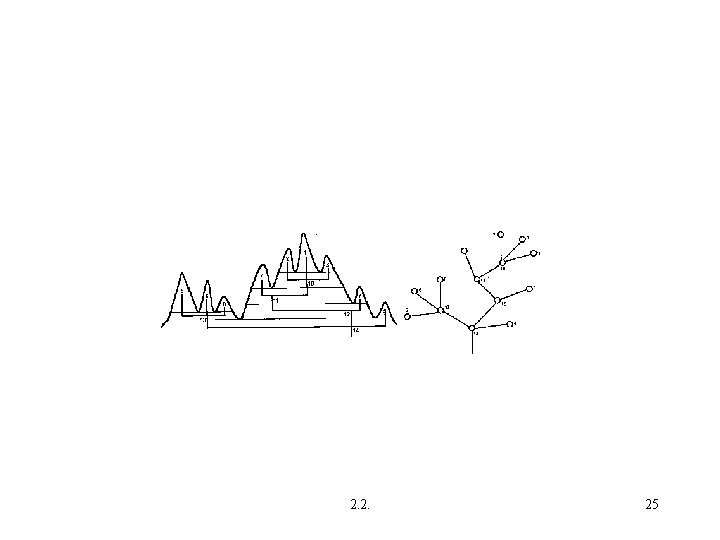
1 2 5 5 3 6 8 4 3 10 4 6 11 10 8 1 2 7 7 13 11 12 12 9 9 14 13 14 2. 2. 24

2. 2. 25

2. 2. 26

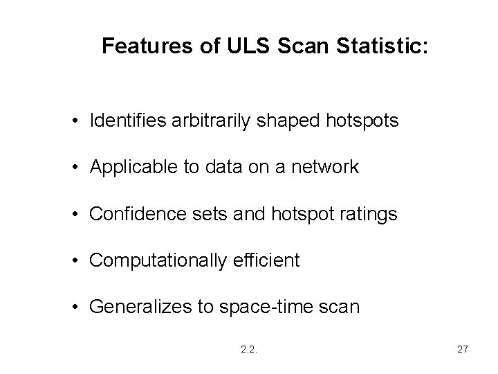
Features of ULS Scan Statistic: • Identifies arbitrarily shaped hotspots • Applicable to data on a network • Confidence sets and hotspot ratings • Computationally efficient • Generalizes to space-time scan 2. 2. 27

2. 2. 28

2. 2. 29

2. 2. 30

2. 2. 31

2. 2. 32

2. 2. 33

2. 2. 34

2. 2. 35

2. 2. 36

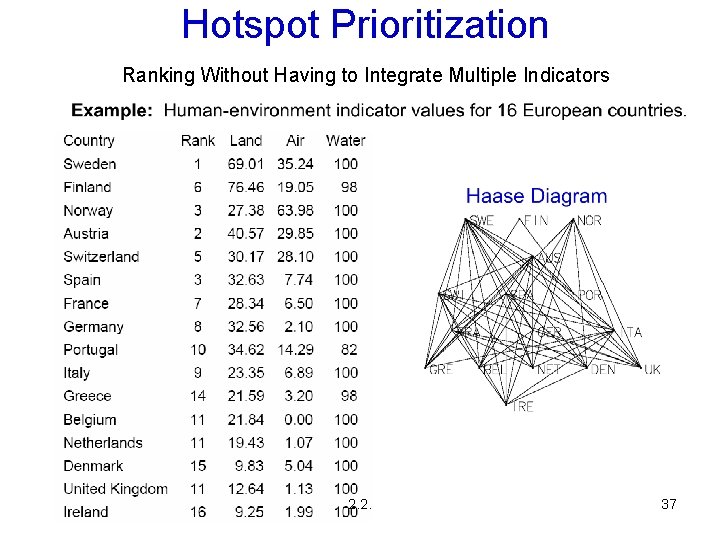
Hotspot Prioritization Ranking Without Having to Integrate Multiple Indicators 2. 2. 37

2. 2. 38

2. 2. 39

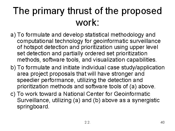
The primary thrust of the proposed work: a) To formulate and develop statistical methodology and computational technology for geoinformatic surveillance of hotspot detection and prioritization using upper level set detection and partially ordered set prioritization methods, software tools, and visualization capabilities. b) To formulate and initiate individual case study/application area project proposals that will have stronger and speedier performance, utilizing the detection and prioritization methods and software tools of (a) above. c) To work toward a National Center for Geoinformatic Surveillance, utilizing (a) and (b) above as a synergistic springboard. 2. 2. 40

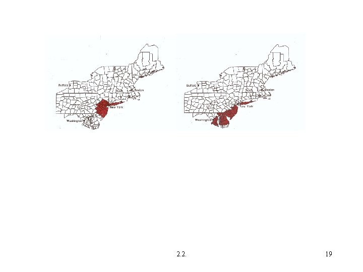
Hotspot Detection Component The hotspot component of the geoinformatic surveillance project is concerned with the question of identifying, delineating, and assessing the significance of hotspots. Our approach to hotspot detection is based on the spatial scan statistic (Kulldorff and Nagarwalla 1995; Kulldorff 1997), which has been widely adopted in the health sciences for disease surveillance. This tends to produce zones that are relatively compact and roughly circular in shape. We propose a novel development of an upper level set (ULS) algorithm for selecting the candidate zones in an adaptive (date-driven) manner. The ULS approach allows for arbitrarily shaped hotspot candidate zones. 2. 2. 41

Hotspot Detection Component Our efforts are driven by a wide variety of case studies of potential interest to Federal agencies involving critical society issues, such as public health, ecosystem health, biosecurity, biosurveillance, robotic networks, social networks, sensor networks, video mining, homeland security, and early warning. For additional information regarding our project, see http: //www. stat. psu. edu/hotspots/, http: //www. stat. psu. edu/~gpp/, demo and poster at this conference, and http: //www. digitalgovernment. org/news/stories/2004/1104_hotspots_heyman. jsp. 2. 2. 42

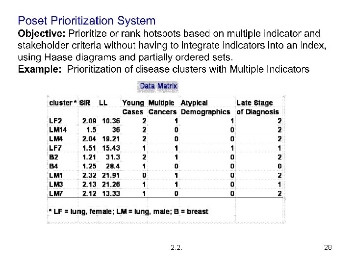
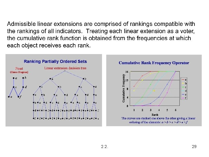
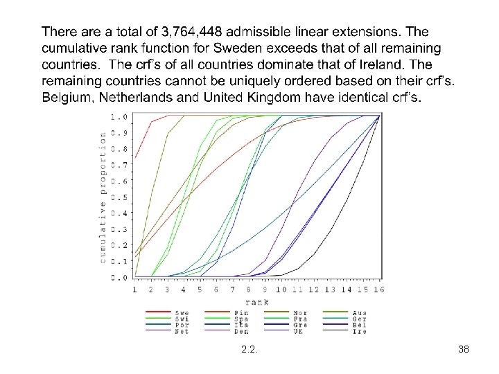
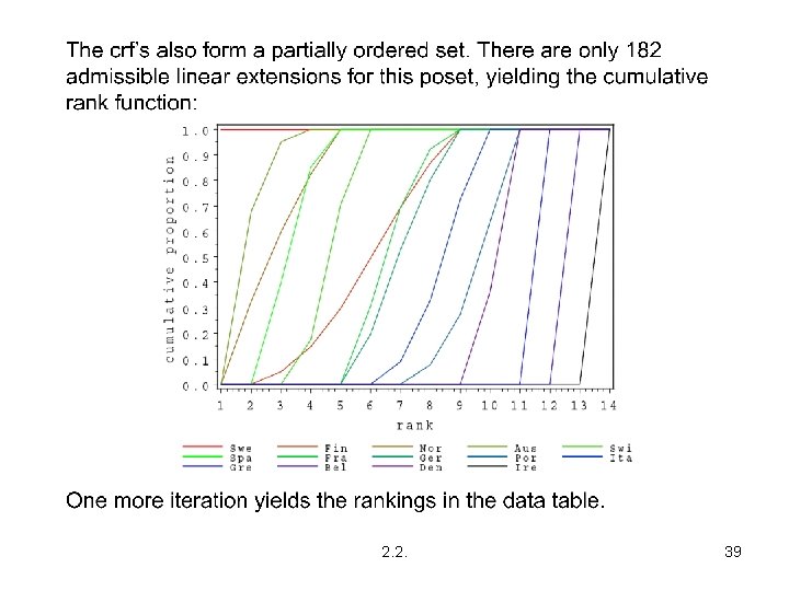
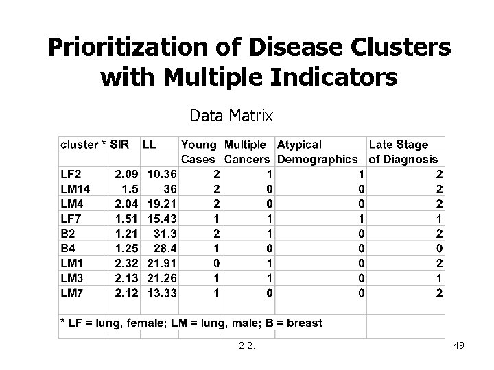
Prioritization Component The prioritization component of the geoinformatic surveillance project is concerned with the question of ranking a finite collection of objects when a suite of indicator values is available for each member of the collection. The goal of the prioritization system is to canonically transform a partial order into a linear order of the objects. We propose a novel prioritization scheme based on multiple indicators that does not require reduction of the data to a single index. 2. 2. 43

Method Upper Level Set (ULS) Scan Statistic for Arbitrarily Shaped Cluster Penn State/NSF/Digital Government 2. 2. 44

Geospatial Surveillance Hotspot Identification and Uncertainty Assessment Penn State/EPA/Atlantic Slope Consortium 2. 2. 45

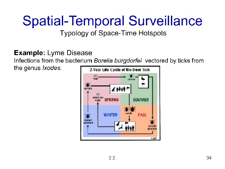
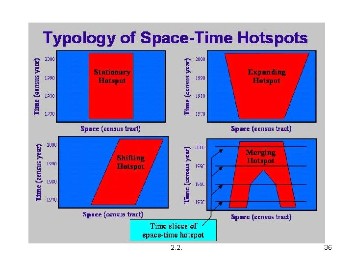
Spatio-Temporal Surveillance Typology of Space-Time Hotspots Penn State/Ford Foundation/Poverty Research 2. 2. 46

Crisis-Index Surveillance Behavior-Event Streams Automata Characterization Penn State/NSF/Digital Government 2. 2. 47

Hotspot Prioritization Ranking Without Having to Integrate the Multiple Indicators Penn State/EPA/Impairment Consortium 2. 2. 48

Prioritization of Disease Clusters with Multiple Indicators Data Matrix 2. 2. 49

ABSTRACT The five year NSF DGP project has been instrumental to conceptualize surveillance geoinformatics partnership among several interested cross-disciplinary scientists in academia, agencies, and private sector. A declared need is around for statistical geoinformatics and software infrastructure for spatial and spatiotemporal hotspot detection. Our efforts are driven by a wide variety of case studies of potential interest to federal agencies involving critical society issues, such as public health, ecosystem health, biosurveillance, biosecurity, sensor networks, robotic networks, social networks, video mining, homeland security, early warning, and disaster management. 2. 2. 50

PARTNERSHIPS • Co. Principal Investigator(s): Raj Acharya; Amy K Glasmeier; Wayne L Myers; Shashi Phoha. • Senior personnel: Robert Brooks; Denice Wardrop; Lance Waller; Elizabeth Middleton; James Shortle; Reza Modarres; Stephen Rathbun; Charles Taillie. • Other collaborators: Howard Burkom; Lawrence Cox; John Kelmelis; Martin Kulldorff; Bo Ranneby; Phil Ross; and others. 2. 2. 51

Training and Development Component Crossdisciplinary classroom for surveillance geoinformatics and multiscale advanced raster map analysis (Ecometrics and Environmetrics). Instructor: G. P. Patil, PI. An advanced crossdisciplinary graduate course across the academic year for graduate students from different programs on the campus, but with common interest in surveillance geoinformatics and multiscale advanced raster map analysis with emphasis on ecometrics and environmetrics. 2. 2. 52

Outreach Component 1. Surveillance Geoinformatics Forum: A partnership in the making. 2. Multiscale Advanced Raster Map Analysis System Partnership: A partnership in the making. 3. Synergistic Outreach 2. 2. 53

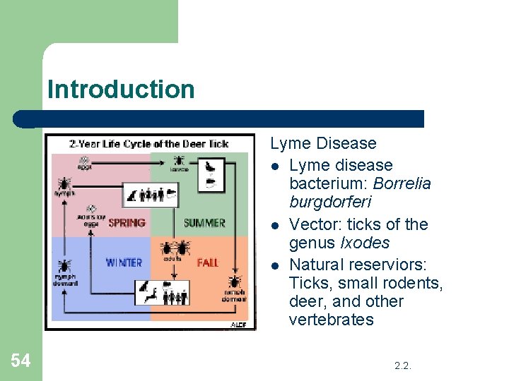
Introduction Lyme Disease l Lyme disease bacterium: Borrelia burgdorferi l Vector: ticks of the genus Ixodes l Natural reserviors: Ticks, small rodents, deer, and other vertebrates 54 2. 2.

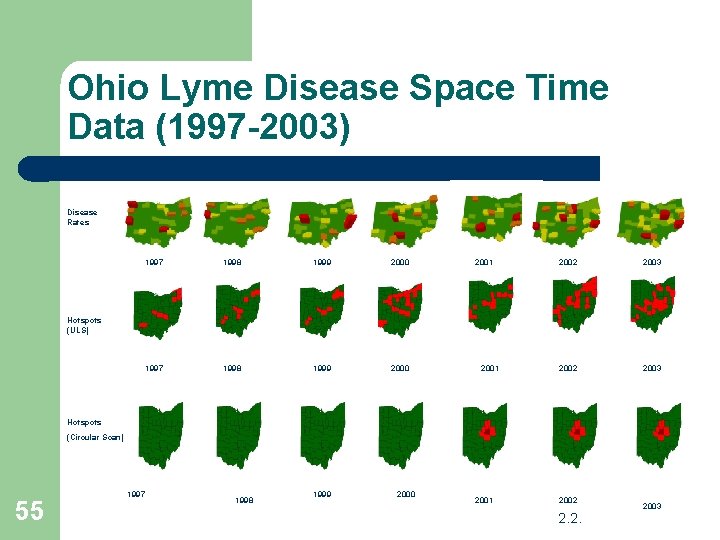
Ohio Lyme Disease Space Time Data (1997 -2003) Disease Rates 1997 1998 1999 2000 2001 2002 2003 Hotspots (ULS) 2001 Hotspots (Circular Scan) 55 1997 1998 1999 2000 2001 2002 2. 2. 2003

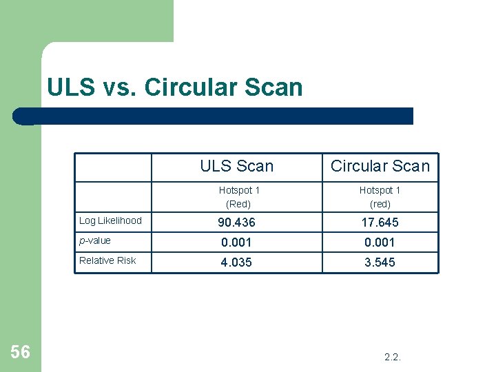
ULS vs. Circular Scan ULS Scan Circular Scan Hotspot 1 (Red) Hotspot 1 (red) 90. 436 17. 645 p-value 0. 001 Relative Risk 4. 035 3. 545 Log Likelihood 56 2. 2.

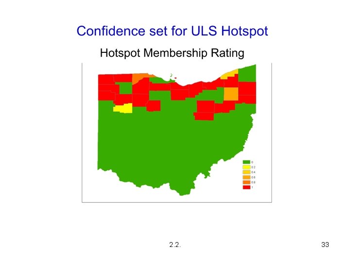
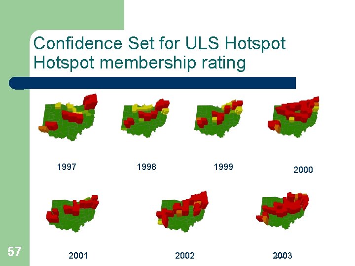
Confidence Set for ULS Hotspot membership rating 1997 57 2001 1998 1999 2002 2000 2. 2. 2003

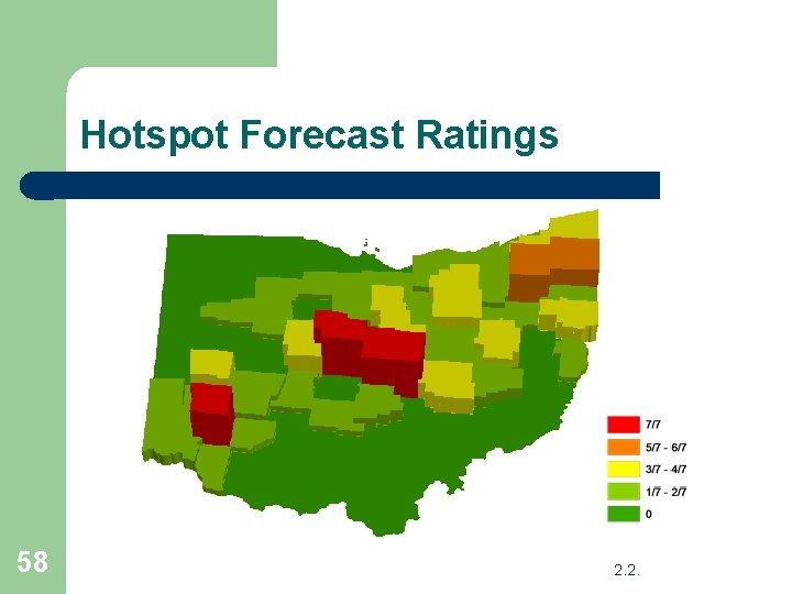
Hotspot Forecast Ratings 58 2. 2.

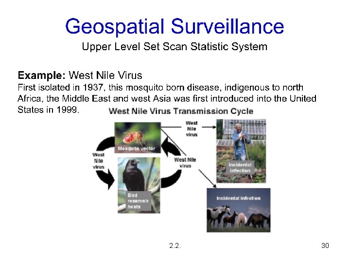
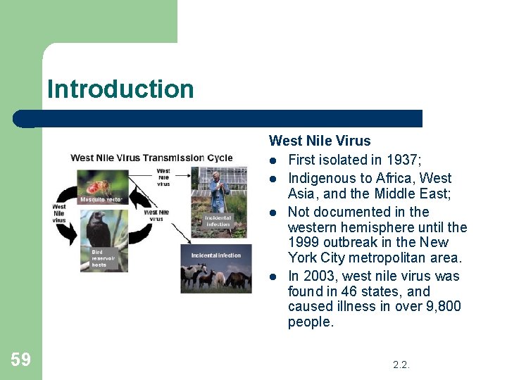
Introduction West Nile Virus l First isolated in 1937; l Indigenous to Africa, West Asia, and the Middle East; l Not documented in the western hemisphere until the 1999 outbreak in the New York City metropolitan area. l In 2003, west nile virus was found in 46 states, and caused illness in over 9, 800 people. 59 2. 2.

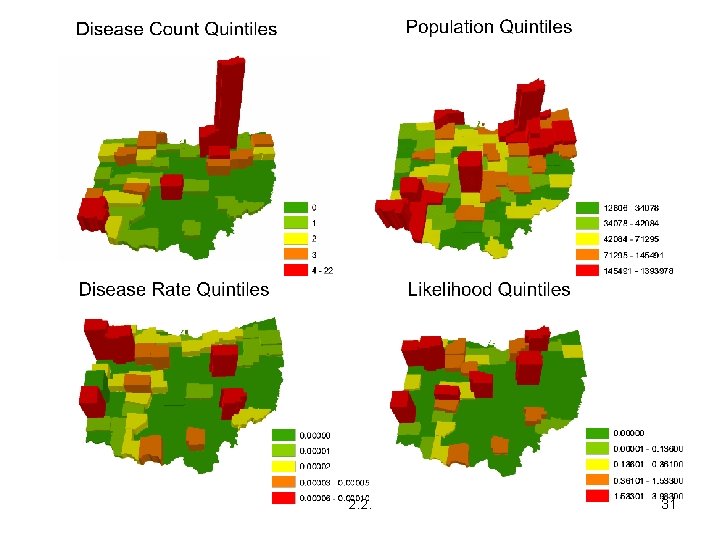
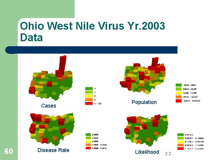
Ohio West Nile Virus Yr. 2003 Data Cases 60 Disease Rate Population Likelihood 2. 2.

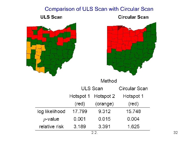
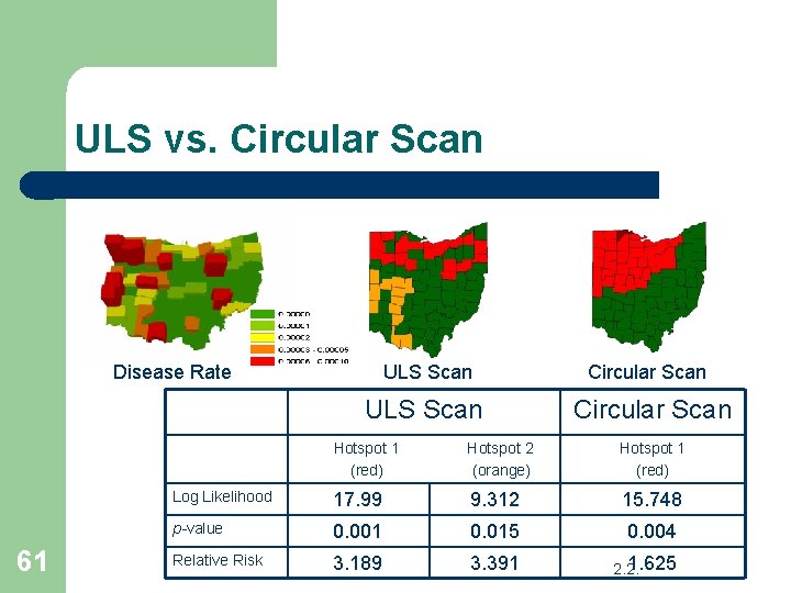
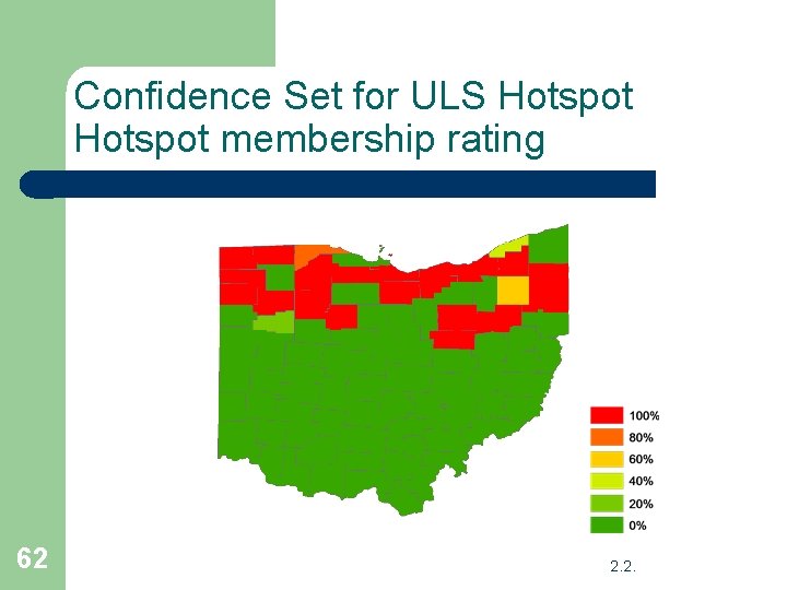
ULS vs. Circular Scan Disease Rate 61 ULS Scan Circular Scan Hotspot 1 (red) Hotspot 2 (orange) Hotspot 1 (red) Log Likelihood 17. 99 9. 312 15. 748 p-value 0. 001 0. 015 0. 004 Relative Risk 3. 189 3. 391 1. 625 2. 2.

Confidence Set for ULS Hotspot membership rating 62 2. 2.

Early Detection of Disease Outbreaks with Applications in New York City Prospective Disease Surveillance n The Spatial Scan Statistic n Dead Birds and West-Nile Virus Surveillance in New York City n Other Current Applications n 2. 2. 63

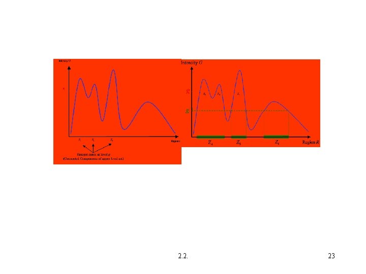
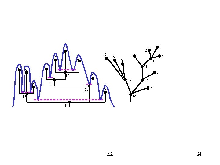
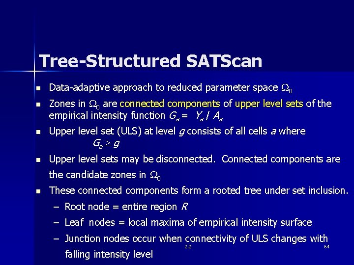
Tree-Structured SATScan n Data-adaptive approach to reduced parameter space 0 n Zones in 0 are connected components of upper level sets of the empirical intensity function Ga = Ya / Aa n n Upper level set (ULS) at level g consists of all cells a where Ga g Upper level sets may be disconnected. Connected components are the candidate zones in 0 n These connected components form a rooted tree under set inclusion. – Root node = entire region R – Leaf nodes = local maxima of empirical intensity surface – Junction nodes occur when connectivity of ULS changes with falling intensity level 2. 2. 64

Benefits Of ULS Scan Statistic Approach Identifies arbitrary shaped clusters n Computationally efficient n Confidence set, hotspot rating n Applicable to continuous response n Generalizes to space-time scan n 2. 2. 65

GEOINFORMATIC SURVEILLANCE Surveillance System For Water Resources n n n Functional Surveillance System Infrastructure Decision Support System Geographical Synoptic and Network-Based Surveillance Natural, Accidental, and/or Intentional Hotspots Prioritization and Ranking Based on Multiple Criteria 2. 2. 66

GEOINFORMATIC SURVEILLANCE Surveillance System For Water Resources n n n Network-Based Analysis of Biological Integrity in Freshwater Streams Critical Area Detection and Prioritization Across Geographical Regions and Networks A Prototype Upper Level Set Scan System in the Making A Novel Innovative Breakthrough at the Door A Part of the Multiscale Advanced Raster Map Analysis System 2. 2. 67

CHESAPEAKE BAY WATERSHED Mid-Atlantic Regional Earth Systems Science Application Center n n n Land Management Biodiversity Management Bay Restoration Geospatial Metrics Spatial and Temporal Hotspot Detection and Prioritization 2. 2. 68

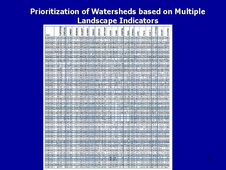
Prioritization of Watersheds based on Multiple Landscape Indicators 2. 2. 69

Combining Environmental Data and Information n n Disparate Sources Satellite, Sites, Samplings Monitoring, Hypothesis Testing, Prioritization Statistical Issues and Approaches Work with Rao, National Medal of Science Recipient 2. 2. 70