Calibration Triangulation and Structure from Motion Thursday 10
Calibration, Triangulation and Structure from Motion Thursday, 10 th October 2019 Samyak Datta Disclaimer: These slides have been borrowed from Derek Hoiem, Kristen Grauman and the Coursera course on Robotic Perception (by Jianbo Shi and Kostas Danilidis). Derek adapted many slides from Lana Lazebnik, Silvio 1 Saverese, Steve Seitz, and took many figures from Hartley & Zisserman.

Reminder • PS 3 is due on 10/16 2
Reminder • PS 3 is due on 10/16 • Project proposals were due last night – 2 project late days – We’ll assign project teams to TAs 3
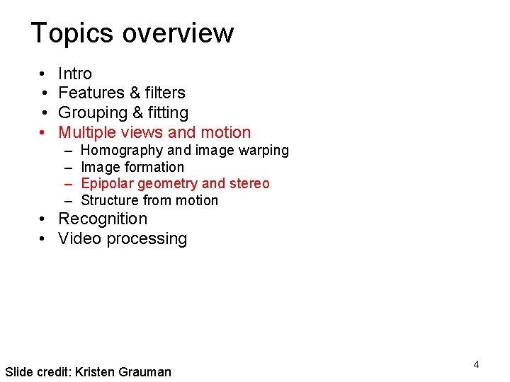
Topics overview • • Intro Features & filters Grouping & fitting Multiple views and motion – – Homography and image warping Image formation Epipolar geometry and stereo Structure from motion • Recognition • Video processing Slide credit: Kristen Grauman 4
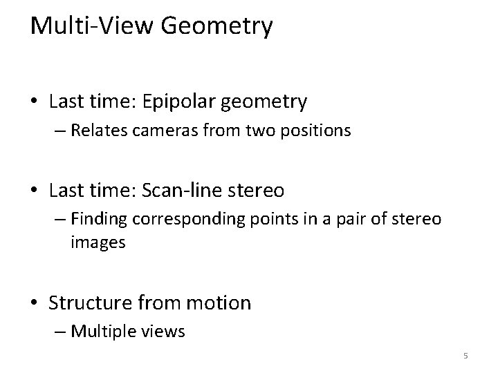
Multi-View Geometry • Last time: Epipolar geometry – Relates cameras from two positions • Last time: Scan-line stereo – Finding corresponding points in a pair of stereo images • Structure from motion – Multiple views 5
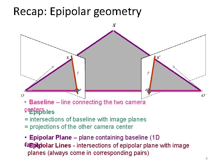
Recap: Epipolar geometry X x x’ • Baseline – line connecting the two camera centers • Epipoles = intersections of baseline with image planes = projections of the other camera center • Epipolar Plane – plane containing baseline (1 D • family) Epipolar Lines - intersections of epipolar plane with image planes (always come in corresponding pairs) 6
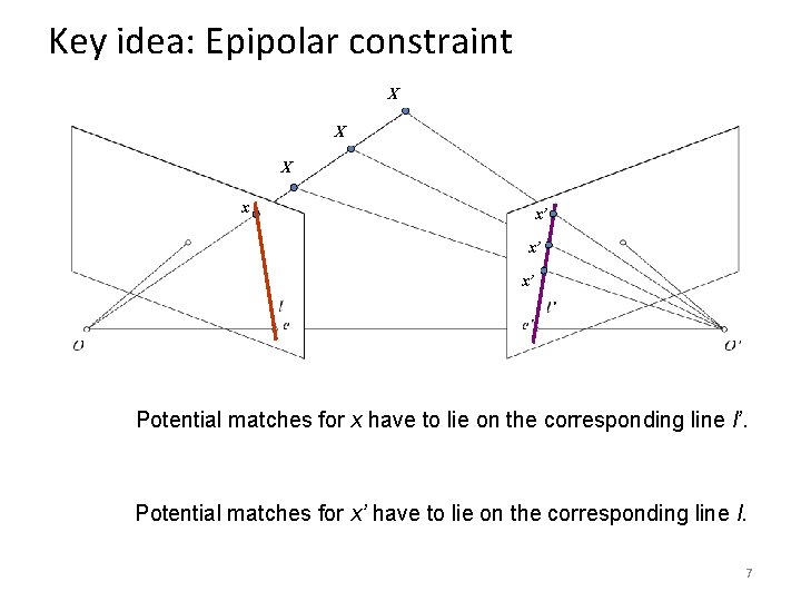
Key idea: Epipolar constraint X X X x x’ x’ x’ Potential matches for x have to lie on the corresponding line l’. Potential matches for x’ have to lie on the corresponding line l. 7
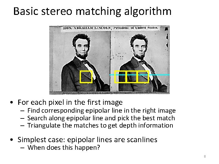
Basic stereo matching algorithm • For each pixel in the first image – Find corresponding epipolar line in the right image – Search along epipolar line and pick the best match – Triangulate the matches to get depth information • Simplest case: epipolar lines are scanlines – When does this happen? 8
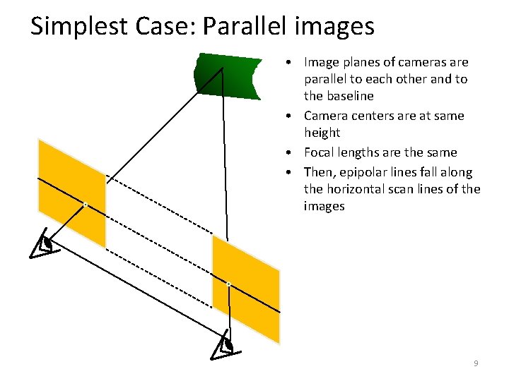
Simplest Case: Parallel images • Image planes of cameras are parallel to each other and to the baseline • Camera centers are at same height • Focal lengths are the same • Then, epipolar lines fall along the horizontal scan lines of the images 9
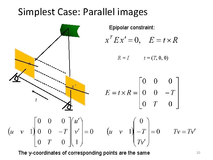
Simplest Case: Parallel images Epipolar constraint: R=I x t = (T, 0, 0) x’ t The y-coordinates of corresponding points are the same 10
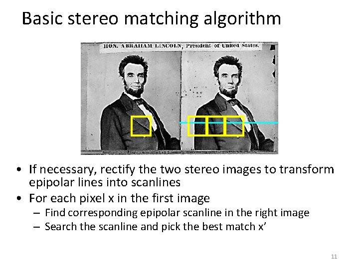
Basic stereo matching algorithm • If necessary, rectify the two stereo images to transform epipolar lines into scanlines • For each pixel x in the first image – Find corresponding epipolar scanline in the right image – Search the scanline and pick the best match x’ 11
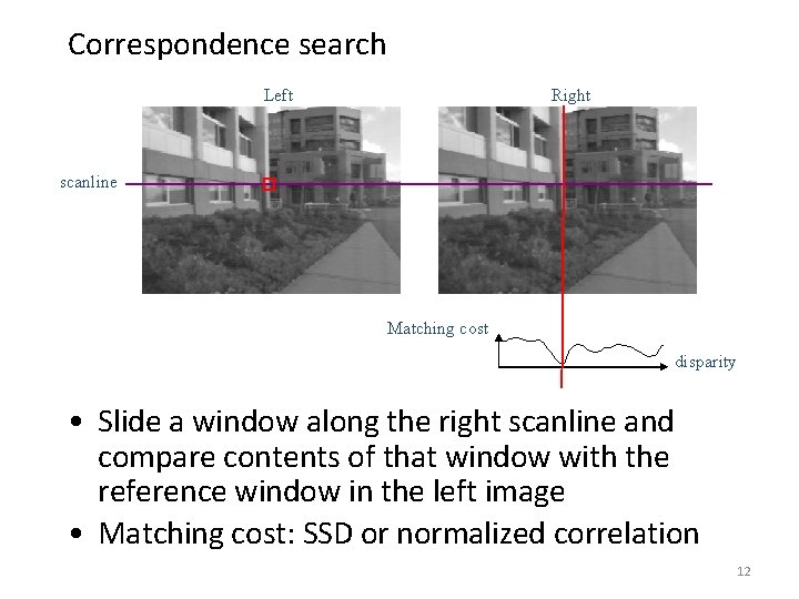
Correspondence search Left Right scanline Matching cost disparity • Slide a window along the right scanline and compare contents of that window with the reference window in the left image • Matching cost: SSD or normalized correlation 12
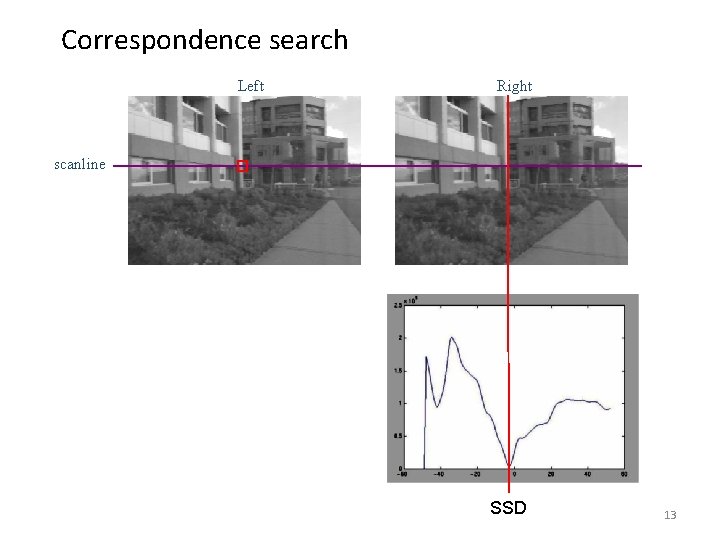
Correspondence search Left Right scanline SSD 13
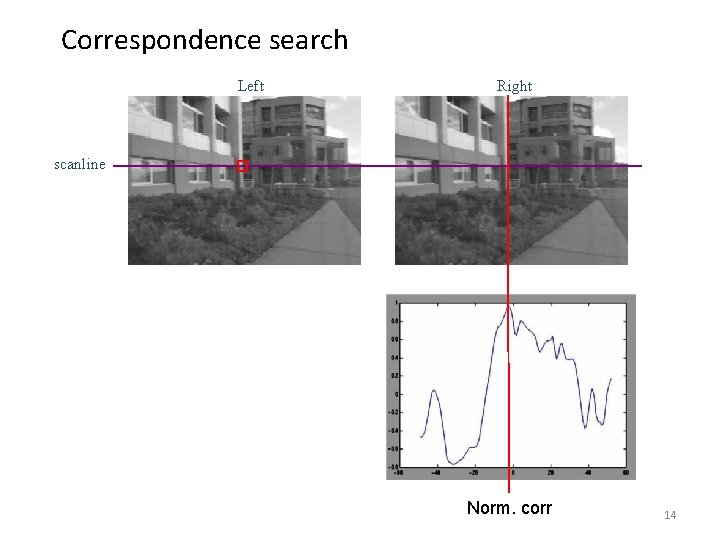
Correspondence search Left Right scanline Norm. corr 14
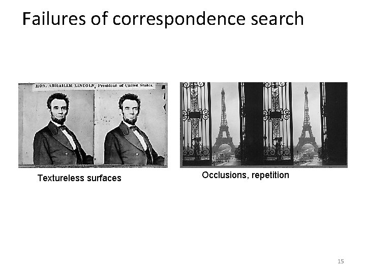
Failures of correspondence search Textureless surfaces Occlusions, repetition 15
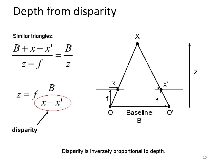
Depth from disparity X Similar triangles: z x x’ f O f Baseline B O’ disparity Disparity is inversely proportional to depth. 16
Topics overview • • Class Intro Features & filters Grouping & fitting Multiple views and motion – – Homography and image warping Image formation Epipolar geometry and stereo Calibration, Triangulation and Structure from motion • Recognition • Video processing Slide credit: Kristen Grauman 17
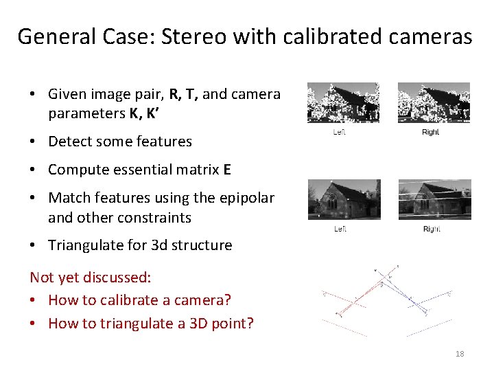
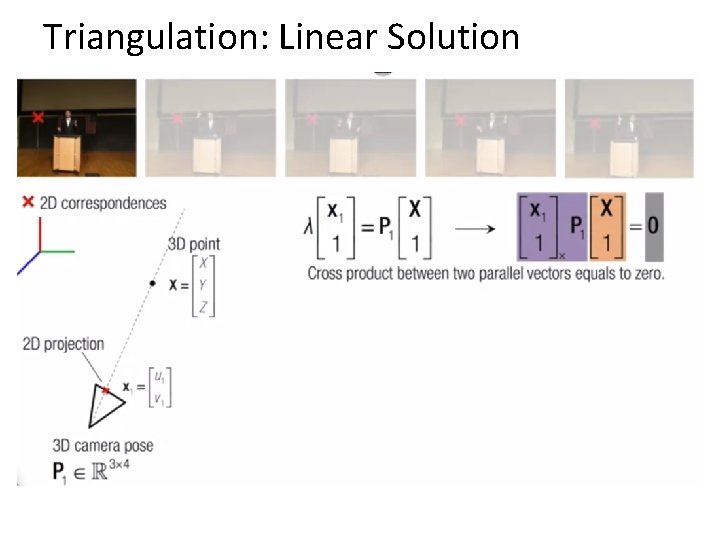
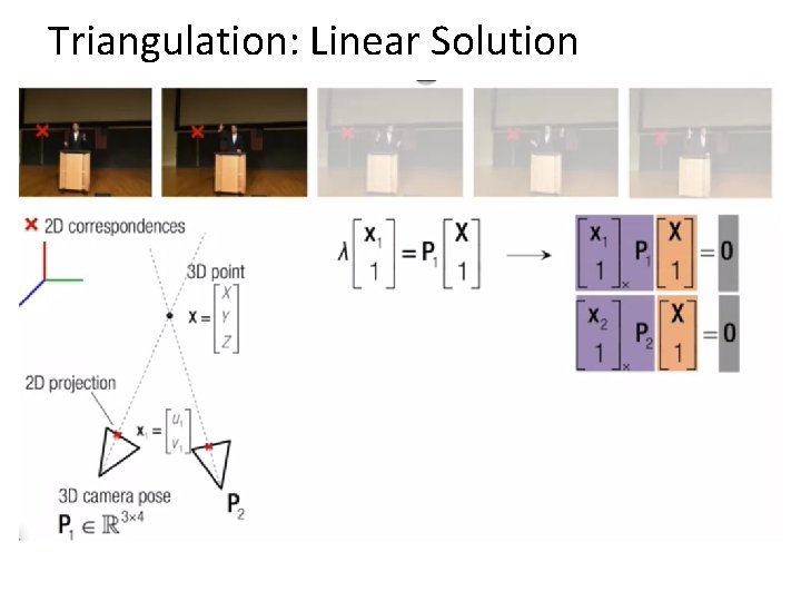
General Case: Stereo with calibrated cameras • Given image pair, R, T, and camera parameters K, K’ • Detect some features • Compute essential matrix E • Match features using the epipolar and other constraints • Triangulate for 3 d structure Not yet discussed: • How to calibrate a camera? • How to triangulate a 3 D point? 18
Today – Calibration – Triangulation – Structure from Motion – Example stereo and Sf. M applications 19
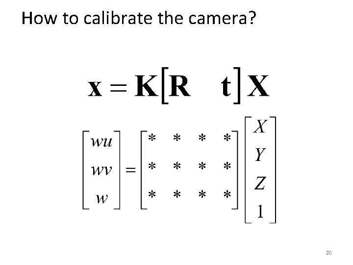
How to calibrate the camera? 20
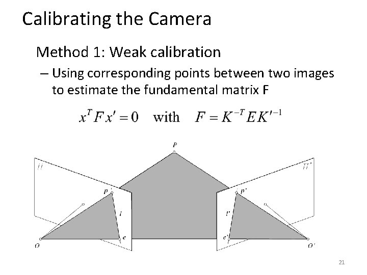
Calibrating the Camera Method 1: Weak calibration – Using corresponding points between two images to estimate the fundamental matrix F 21
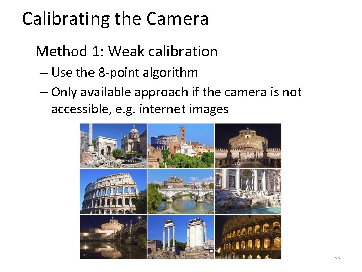
Calibrating the Camera Method 1: Weak calibration – Use the 8 -point algorithm – Only available approach if the camera is not accessible, e. g. internet images 22
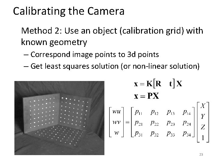
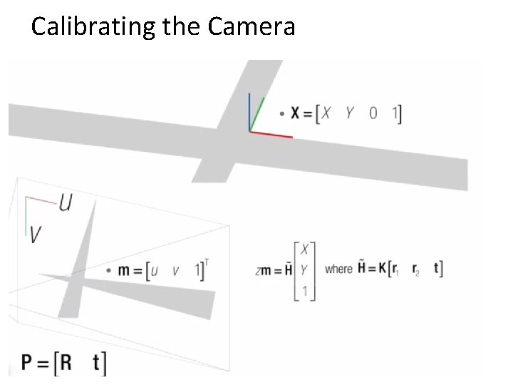
Calibrating the Camera Method 2: Use an object (calibration grid) with known geometry – Correspond image points to 3 d points – Get least squares solution (or non-linear solution) 23
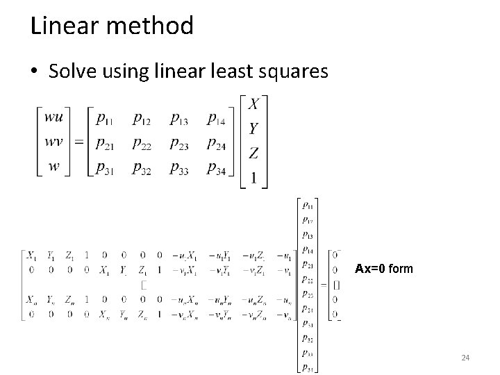
Linear method • Solve using linear least squares Ax=0 form 24
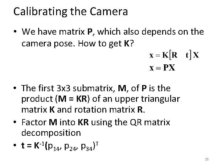
Calibrating the Camera • We have matrix P, which also depends on the camera pose. How to get K? • The first 3 x 3 submatrix, M, of P is the product (M = KR) of an upper triangular matrix K and rotation matrix R. • Factor M into KR using the QR matrix decomposition • t = K-1(p 14, p 24, p 34)T 25
Calibration with linear method • Advantages: easy to formulate and solve • Disadvantages – Doesn’t tell you camera parameters – Can’t impose constraints, such as known focal length – Doesn’t minimize projection error • Non-linear methods are preferred – Define error as difference between projected points and measured points – Minimize error using Newton’s method or other non-linear optimization – Use linear method for initialization 26
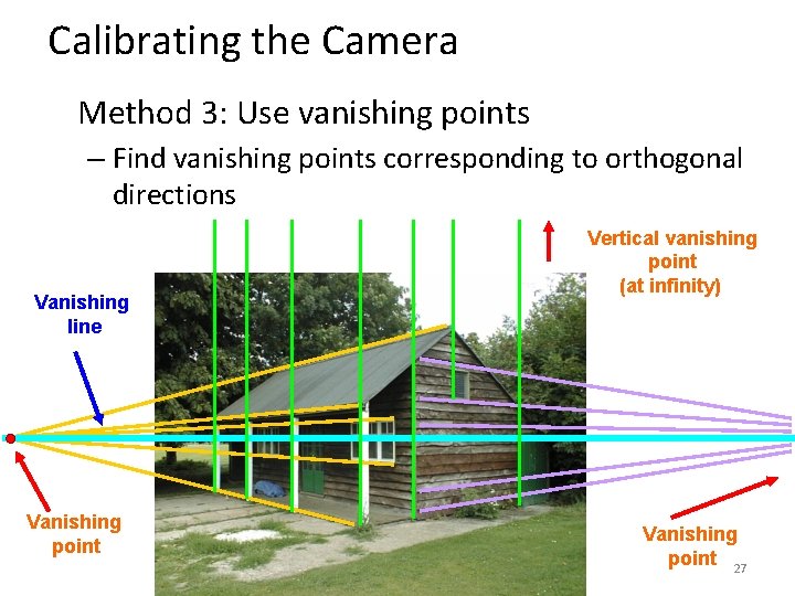
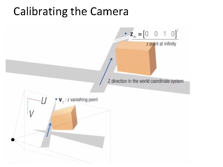
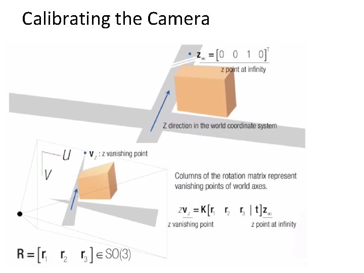
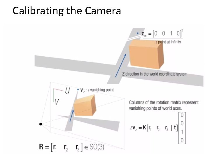
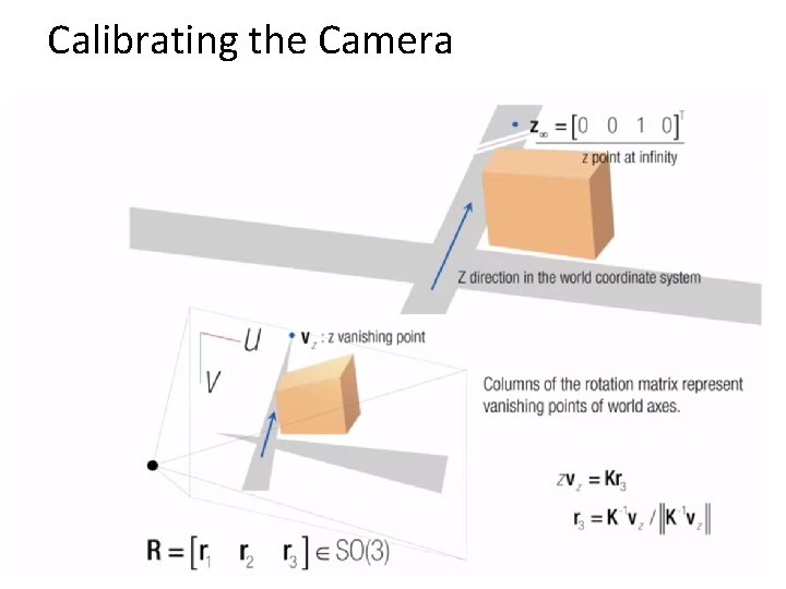
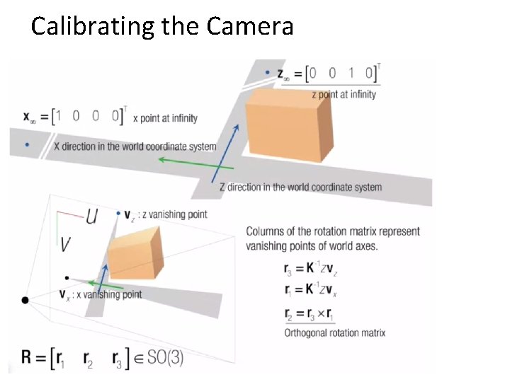
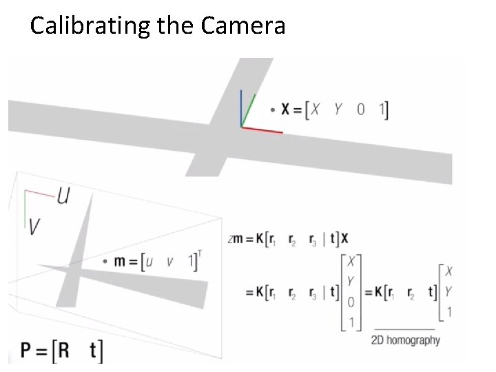
Calibrating the Camera Method 3: Use vanishing points – Find vanishing points corresponding to orthogonal directions Vanishing line Vanishing point Vertical vanishing point (at infinity) Vanishing point 27
Calibrating the Camera
Calibrating the Camera
Calibrating the Camera
Calibrating the Camera
Calibrating the Camera
Calibrating the Camera
Calibrating the Camera
Today – Calibration – Triangulation – Structure from Motion – Example stereo and Sf. M applications 35
Triangulation: Linear Solution
Triangulation: Linear Solution
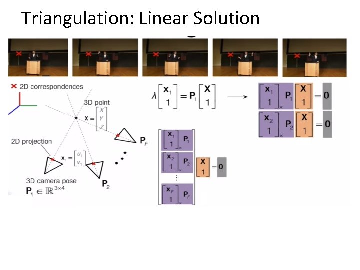
Triangulation: Linear Solution
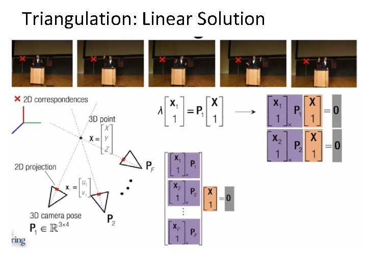
Triangulation: Linear Solution
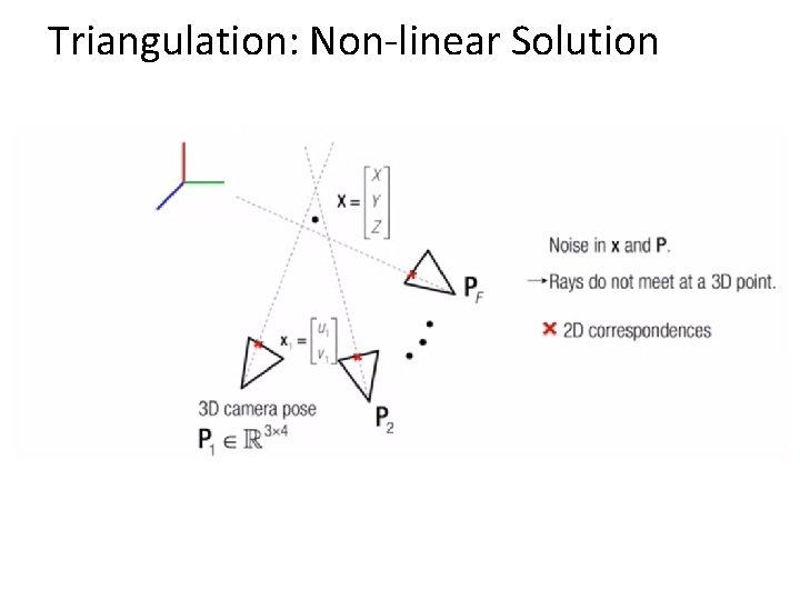
Triangulation: Non-linear Solution
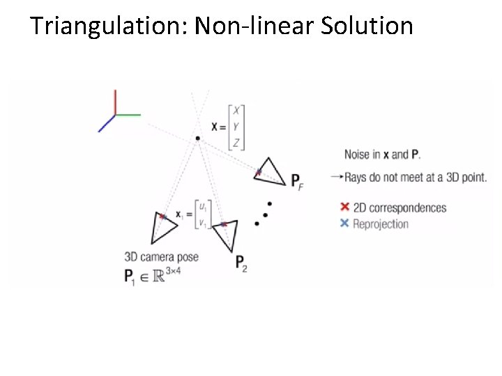
Triangulation: Non-linear Solution
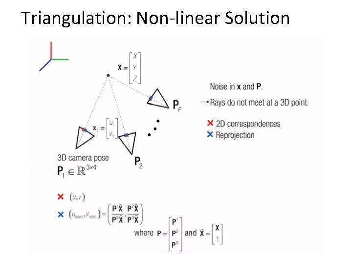
Triangulation: Non-linear Solution
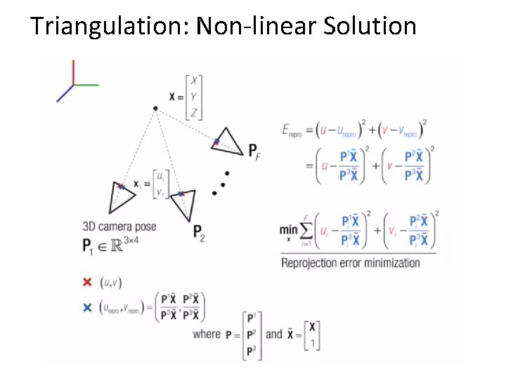
Triangulation: Non-linear Solution
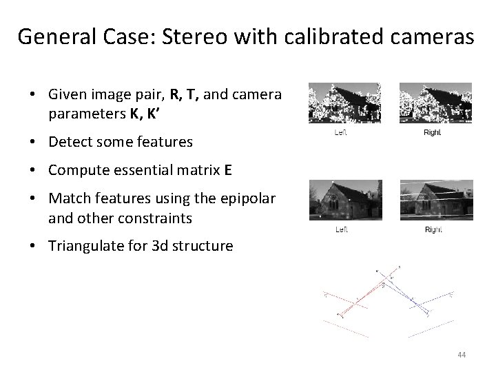
General Case: Stereo with calibrated cameras • Given image pair, R, T, and camera parameters K, K’ • Detect some features • Compute essential matrix E • Match features using the epipolar and other constraints • Triangulate for 3 d structure 44
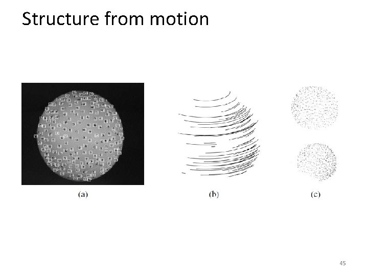
Structure from motion 45
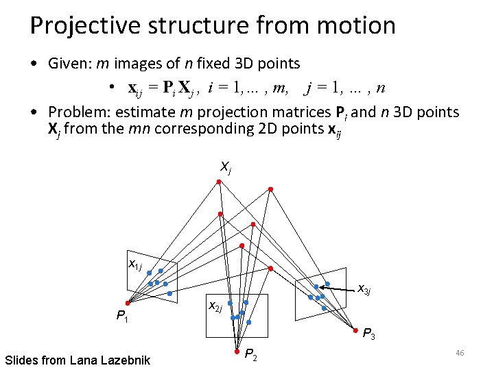
Projective structure from motion • Given: m images of n fixed 3 D points • xij = Pi Xj , i = 1, … , m, j = 1, … , n • Problem: estimate m projection matrices Pi and n 3 D points Xj from the mn corresponding 2 D points xij Xj x 1 j x 3 j P 1 x 2 j P 3 Slides from Lana Lazebnik P 2 46
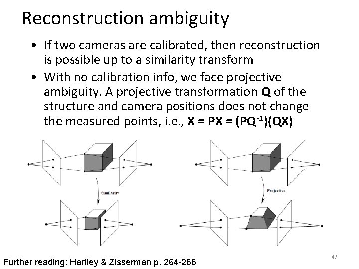
Reconstruction ambiguity • If two cameras are calibrated, then reconstruction is possible up to a similarity transform • With no calibration info, we face projective ambiguity. A projective transformation Q of the structure and camera positions does not change the measured points, i. e. , X = PX = (PQ-1)(QX) Further reading: Hartley & Zisserman p. 264 -266 47
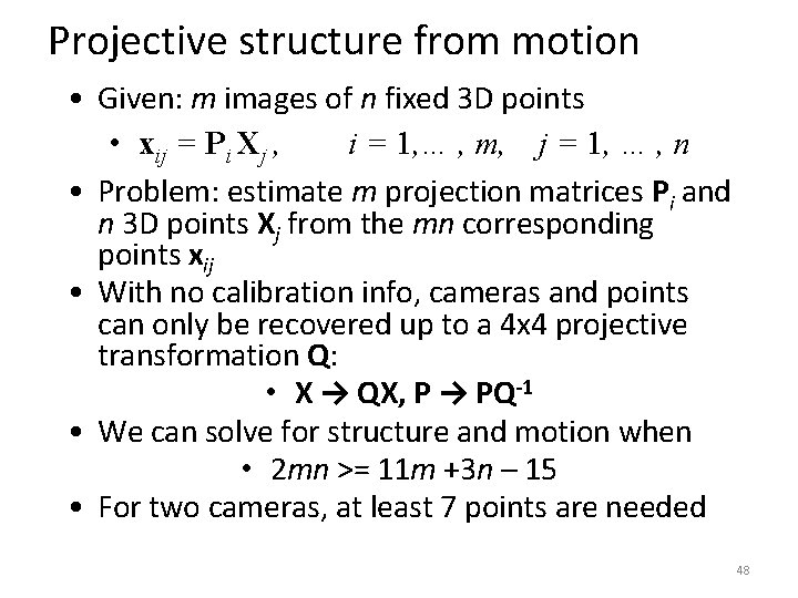
Projective structure from motion • Given: m images of n fixed 3 D points • xij = Pi Xj , i = 1, … , m, j = 1, … , n • Problem: estimate m projection matrices Pi and n 3 D points Xj from the mn corresponding points xij • With no calibration info, cameras and points can only be recovered up to a 4 x 4 projective transformation Q: • X → QX, P → PQ-1 • We can solve for structure and motion when • 2 mn >= 11 m +3 n – 15 • For two cameras, at least 7 points are needed 48
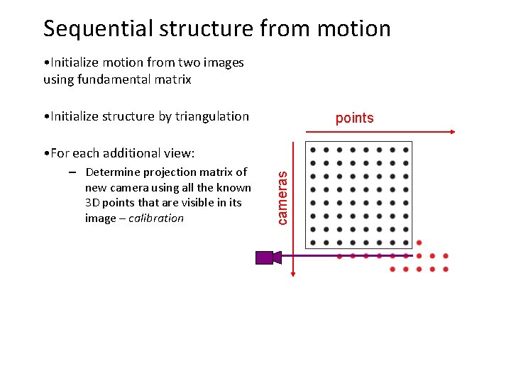
Sequential structure from motion • Initialize motion from two images using fundamental matrix • Initialize structure by triangulation points – Determine projection matrix of new camera using all the known 3 D points that are visible in its image – calibration cameras • For each additional view:
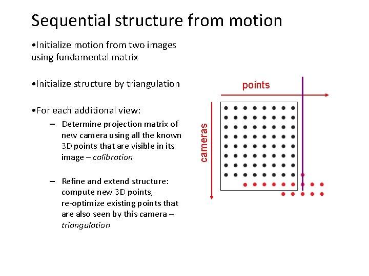
Sequential structure from motion • Initialize motion from two images using fundamental matrix • Initialize structure by triangulation points – Determine projection matrix of new camera using all the known 3 D points that are visible in its image – calibration – Refine and extend structure: compute new 3 D points, re-optimize existing points that are also seen by this camera – triangulation cameras • For each additional view:
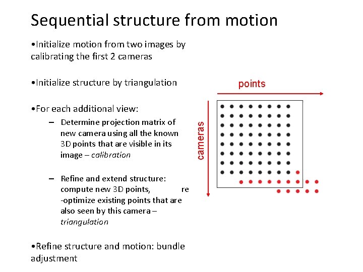
Sequential structure from motion • Initialize motion from two images by calibrating the first 2 cameras • Initialize structure by triangulation points – Determine projection matrix of new camera using all the known 3 D points that are visible in its image – calibration – Refine and extend structure: compute new 3 D points, re -optimize existing points that are also seen by this camera – triangulation • Refine structure and motion: bundle adjustment cameras • For each additional view:
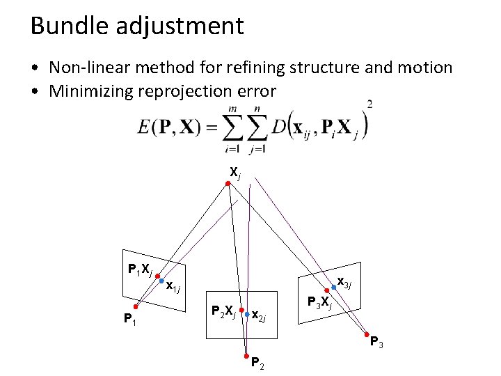
Bundle adjustment • Non-linear method for refining structure and motion • Minimizing reprojection error Xj P 1 x 3 j x 1 j P 2 Xj x 2 j P 3 Xj P 3 P 2
Today – Calibration – Triangulation – Structure from Motion – Example stereo and Sf. M applications 53
3 D from multiple images • http: //grail. cs. washington. edu/rome/ 54 Building Rome in a Day: Agarwal et al. 2009

Virtual environments for AI https: //aihabitat. org 55
Topics overview • • Class Intro Features & filters Grouping & fitting Multiple views and motion – – Homography and image warping Image formation Epipolar geometry and stereo Structure from motion • Recognition • Video processing Slide credit: Kristen Grauman 56
- Slides: 56