
CALIBRATION Derek Karssenberg Utrecht University the Netherlands Example

CALIBRATION Derek Karssenberg Utrecht University, the Netherlands
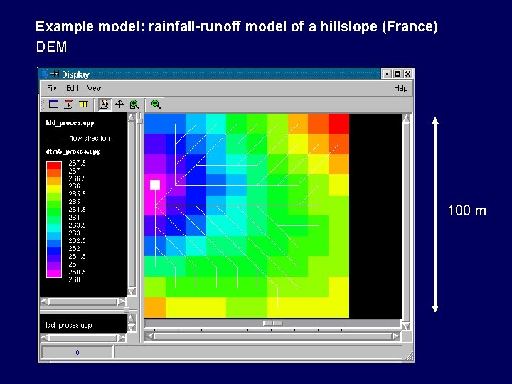
Example model: rainfall-runoff model of a hillslope (France) DEM 100 m
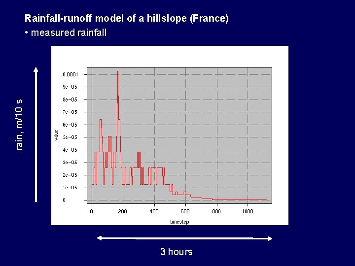
rain, m/10 s Rainfall-runoff model of a hillslope (France) • measured rainfall 3 hours
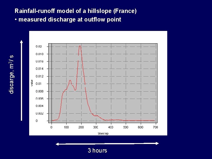
discarge, m 3/ s Rainfall-runoff model of a hillslope (France) • measured discharge at outflow point 3 hours
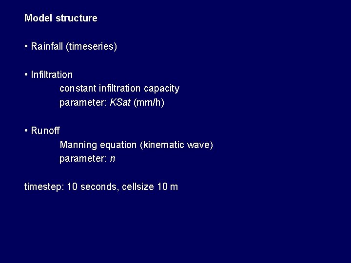
Model structure • Rainfall (timeseries) • Infiltration constant infiltration capacity parameter: KSat (mm/h) • Runoff Manning equation (kinematic wave) parameter: n timestep: 10 seconds, cellsize 10 m
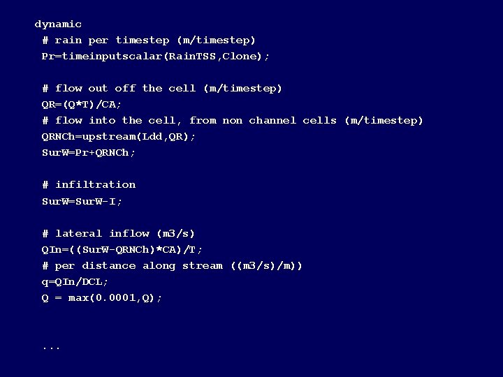
dynamic # rain per timestep (m/timestep) Pr=timeinputscalar(Rain. TSS, Clone); # flow out off the cell (m/timestep) QR=(Q*T)/CA; # flow into the cell, from non channel cells (m/timestep) QRNCh=upstream(Ldd, QR); Sur. W=Pr+QRNCh; # infiltration Sur. W=Sur. W-I; # lateral inflow (m 3/s) QIn=((Sur. W-QRNCh)*CA)/T; # per distance along stream ((m 3/s)/m)) q=QIn/DCL; Q = max(0. 0001, Q); . . .
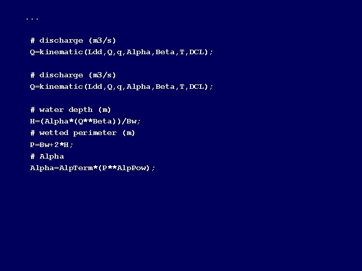
. . . # discharge (m 3/s) Q=kinematic(Ldd, Q, q, Alpha, Beta, T, DCL); # water depth (m) H=(Alpha*(Q**Beta))/Bw; # wetted perimeter (m) P=Bw+2*H; # Alpha=Alp. Term*(P**Alp. Pow);
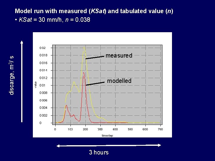
discarge, m 3/ s Model run with measured (KSat) and tabulated value (n) • KSat = 30 mm/h, n = 0. 038 measured modelled 3 hours
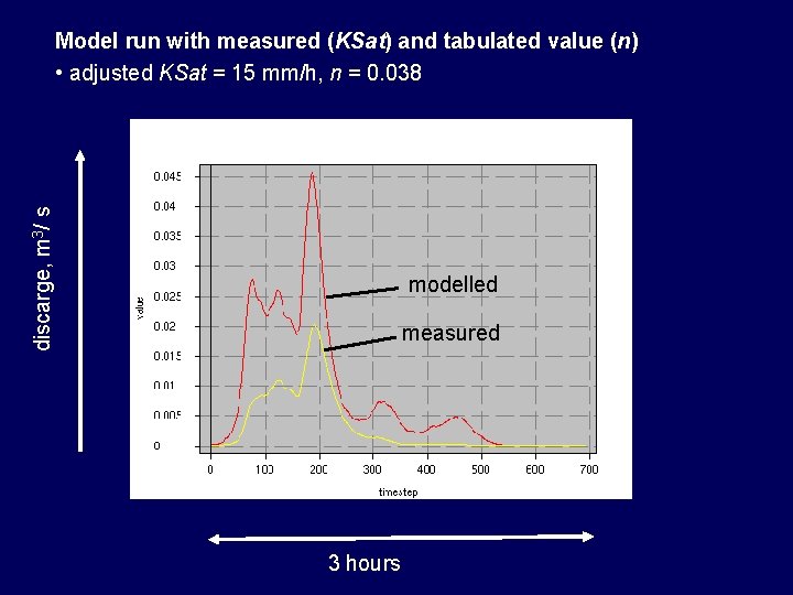
discarge, m 3/ s Model run with measured (KSat) and tabulated value (n) • adjusted KSat = 15 mm/h, n = 0. 038 measured modelled measured 3 hours
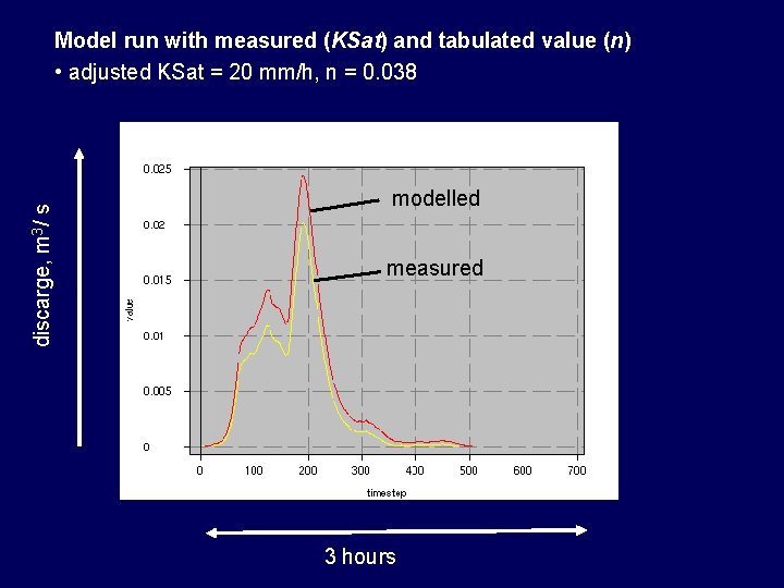
discarge, m 3/ s Model run with measured (KSat) and tabulated value (n) • adjusted KSat = 20 mm/h, n = 0. 038 modelled measured 3 hours
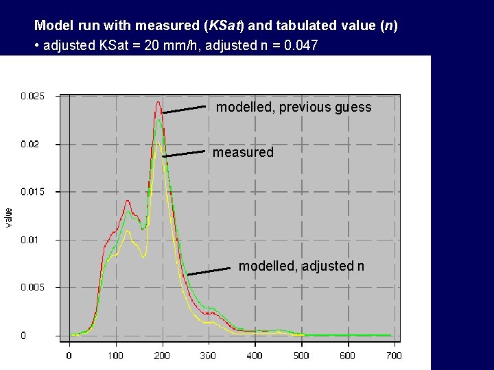
Model run with measured (KSat) and tabulated value (n) • adjusted KSat = 20 mm/h, adjusted n = 0. 047 modelled, previous guess measured modelled, adjusted n 3 hours

Calibration Finding inputs or parameters by minimizing the difference between model outputs and measurements of these outputs z 1. . m i 1. . n f 1. . m p o 1. . m state variables 1. . n inputs 1. . m functionals parameters outputs i. e. a set of state variables in which the interest lies
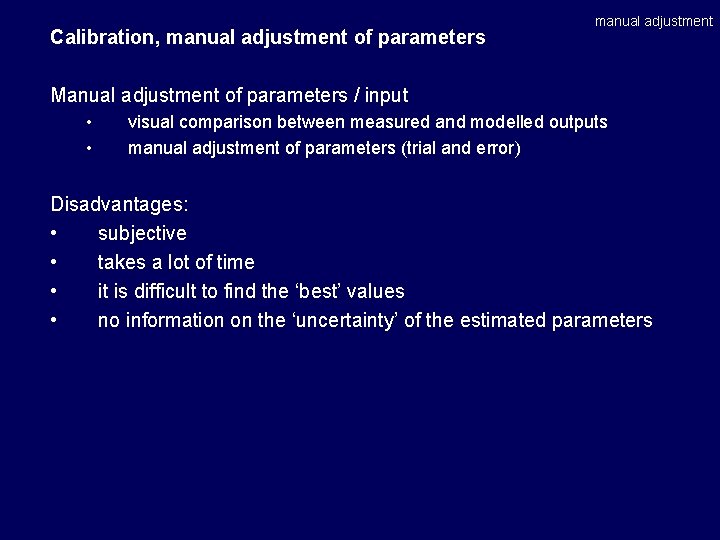
Calibration, manual adjustment of parameters manual adjustment Manual adjustment of parameters / input • • visual comparison between measured and modelled outputs manual adjustment of parameters (trial and error) Disadvantages: • subjective • takes a lot of time • it is difficult to find the ‘best’ values • no information on the ‘uncertainty’ of the estimated parameters
Calibration, automatic adjustment introduction Approach: define a goal function optimize the parameters resulting in the lowest (highest) value of the goal function optimization is done with a computer algorithm
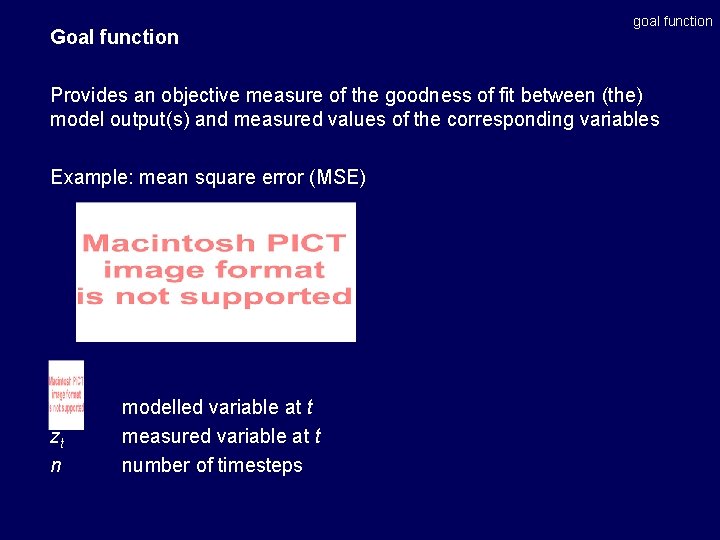
Goal function goal function Provides an objective measure of the goodness of fit between (the) model output(s) and measured values of the corresponding variables Example: mean square error (MSE) zt n modelled variable at t measured variable at t number of timesteps

MSE in our example zt n modelled discharge (m 3/s) at t measured discharge (m 3/s) at t number of timesteps, 691 (each time step is 5 s) goal function
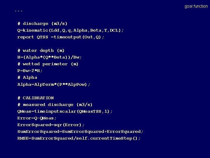
. . . # discharge (m 3/s) Q=kinematic(Ldd, Q, q, Alpha, Beta, T, DCL); report QTSS =timeoutput(Out, Q); # water depth (m) H=(Alpha*(Q**Beta))/Bw; # wetted perimeter (m) P=Bw+2*H; # Alpha=Alp. Term*(P**Alp. Pow); # CALIBRATION # measured discharge (m 3/s) QMeas=timeinputscalar(QMeas. TSS, 1); Error=Q-QMeas; Error. Squared=sqr(Error); Sum. Error. Squared=Sum. Error. Squared+Error. Squared; RMSE=Sum. Error. Squared/self. current. Time. Step(); goal function
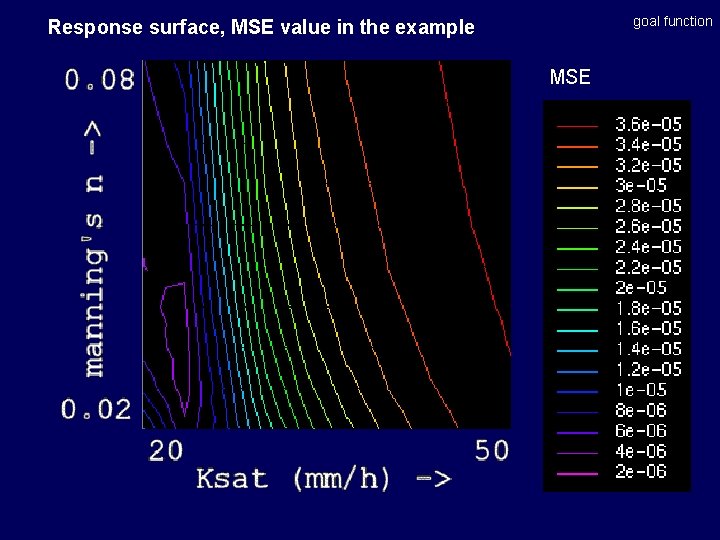
goal function Response surface, MSE value in the example MSE
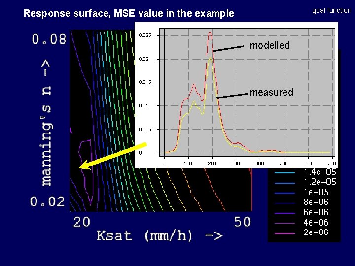
goal function Response surface, MSE value in the example MSE modelled measured
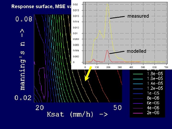
introduction Response surface, MSE value in the example measured MSE modelled
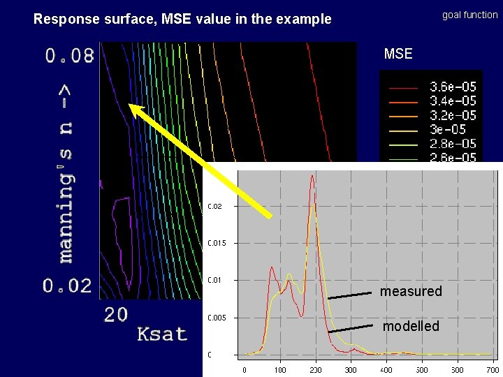
goal function Response surface, MSE value in the example MSE measured modelled
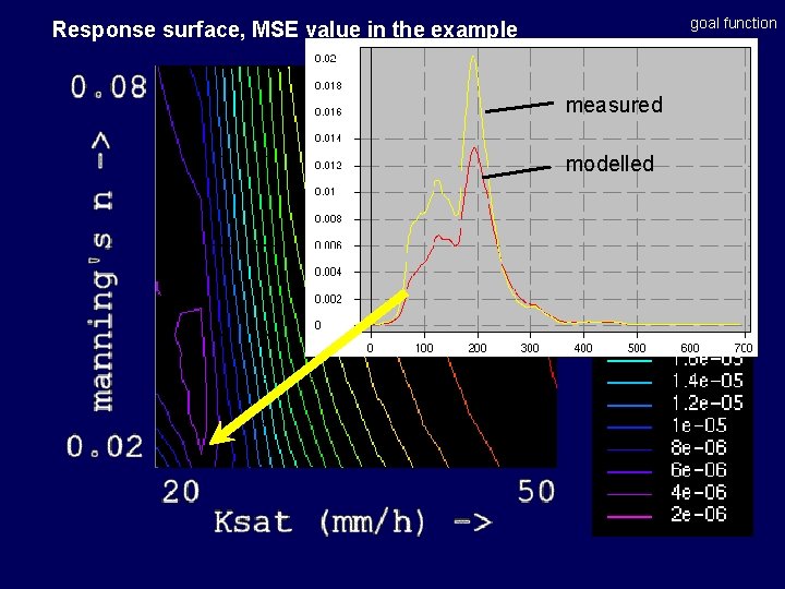
goal function Response surface, MSE value in the example MSE measured modelled
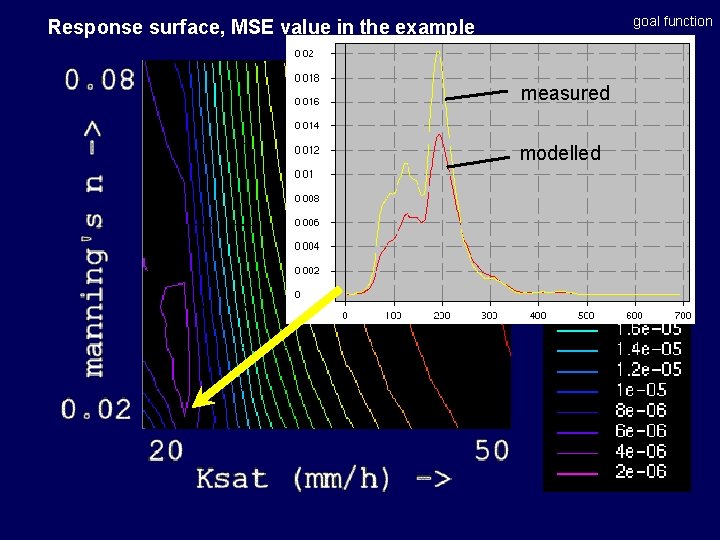
goal function Response surface, MSE value in the example MSE measured modelled
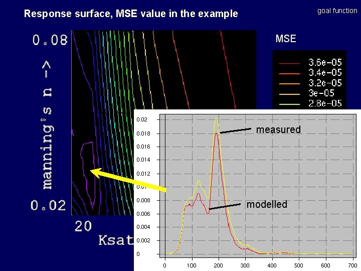
goal function Response surface, MSE value in the example MSE measured modelled
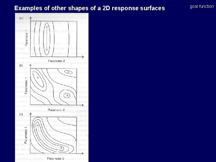
Examples of other shapes of a 2 D response surfaces goal function
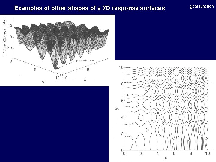
Examples of other shapes of a 2 D response surfaces goal function
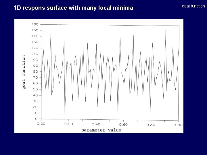
1 D respons surface with many local minima goal function
Higher-dimensional response surfaces When several parameters are unknown, e. g. - saturated conductivity of several soil layers - vegetation cover of several vegetation units - maximum interception store - surface storage of several soil units - manning’s - groundwater flow parameters - etc. . goal function
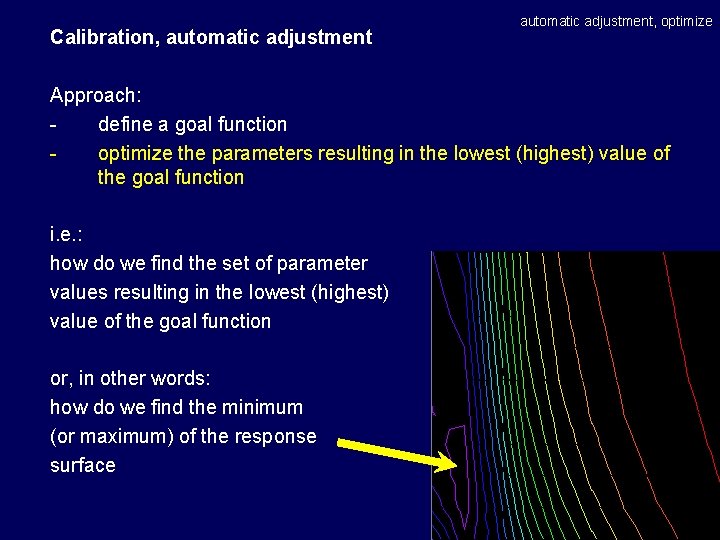
Calibration, automatic adjustment, optimize Approach: define a goal function optimize the parameters resulting in the lowest (highest) value of the goal function i. e. : how do we find the set of parameter values resulting in the lowest (highest) value of the goal function or, in other words: how do we find the minimum (or maximum) of the response surface
Calibration, automatic adjustment, optimize Approach: define a goal function optimize the parameters resulting in the lowest (highest) value of the goal function optimization is done with a computer algorithm - brute force hill-climbing techniques genetic algorithms
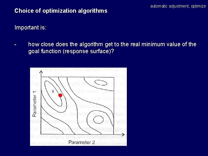
Choice of optimization algorithms automatic adjustment, optimize Important is: - how close does the algorithm get to the real minimum value of the goal function (response surface)?

Choice of optimization algorithms automatic adjustment, optimize Important is: - how close does the algorithm get to the real minimum value of the goal function (response surface)? - is the global minimum found or just a local minimum?
Choice of optimization algorithms automatic adjustment, optimize Important is: - how close does the algorithm get to the real minimum value of the goal function (response surface)? - is the global minimum found or just a local minimum? - how many model runs are needed to find the minimum?
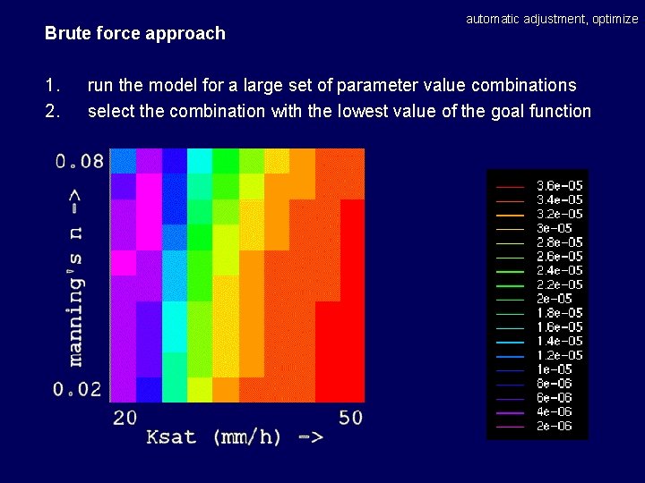
Brute force approach 1. 2. automatic adjustment, optimize run the model for a large set of parameter value combinations select the combination with the lowest value of the goal function
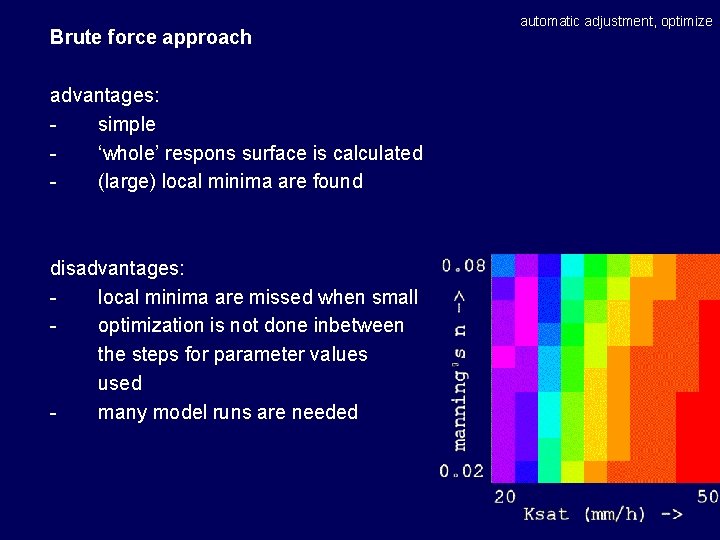
Brute force approach advantages: simple ‘whole’ respons surface is calculated (large) local minima are found disadvantages: local minima are missed when small optimization is not done inbetween the steps for parameter values used many model runs are needed automatic adjustment, optimize
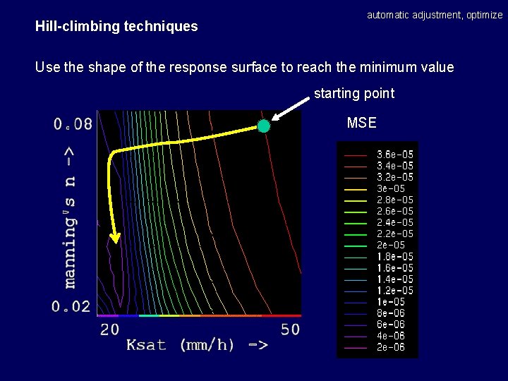
Hill-climbing techniques automatic adjustment, optimize Use the shape of the response surface to reach the minimum value starting point MSE
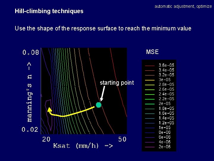
automatic adjustment, optimize Hill-climbing techniques Use the shape of the response surface to reach the minimum value MSE starting point
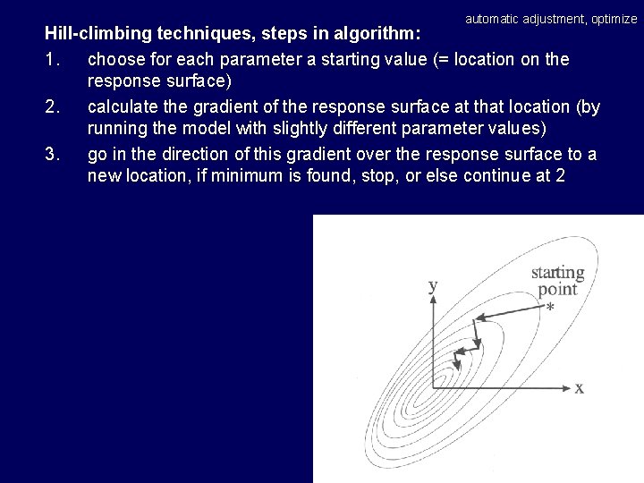
automatic adjustment, optimize Hill-climbing techniques, steps in algorithm: 1. choose for each parameter a starting value (= location on the response surface) 2. calculate the gradient of the response surface at that location (by running the model with slightly different parameter values) 3. go in the direction of this gradient over the response surface to a new location, if minimum is found, stop, or else continue at 2
automatic adjustment, optimize Hill-climbing techniques advantages: small number of runs needed (compared to brute force) location of minimum can be found with high precision
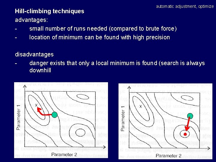
automatic adjustment, optimize Hill-climbing techniques advantages: small number of runs needed (compared to brute force) location of minimum can be found with high precision disadvantages danger exists that only a local minimum is found (search is always downhill
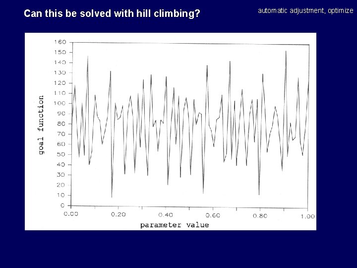
Can this be solved with hill climbing? automatic adjustment, optimize
Genetic algorithm automatic adjustment, optimize Uses analogy with biological evolution: - individual: one parameter set coded as a binary string - population: several individuals (several parameter sets) - population evolves until individuals emerge that represent a very low (high) value of the objective function - evolution by selection, cross-over and mutation

automatic adjustment, optimize . model objective function
Genetic algorithms automatic adjustment, optimize advantages: capable to search in many local minima relatively small number of model runs (compared to brute force) disadvantages not possible (or very difficult) to describe the value of the outcome by means of statistics
Choice of the optimization algorithm automatic adjustment, optimize simple problems: brute force hill climbing approach - standard software available (PEST) multiple local minima: genetic algorithm or combination of hill climbing and genetic algorithm
- Slides: 45