Calculus Crash Course Physics Rushin through the Basics

Calculus Crash Course Physics Rushin’ through the Basics for

The Two Main Problems of Calculus: The Tangent line problem – Find the instantaneous slope of a curve by finding the line tangent to the curve at that point The Area problem – finding the area bound beneath some curve

Why the Tangent Line Problem is important to physics Slopes always indicate the rate at which one variable is changing as another variable is changing too. The rate at which quantities like position, velocity, force, mass, and energy change with time are important values to know when performing certain physics calculations. Calculus will allow us to measure these rates even if they are not constant but instead are continuously changing.

v. time graph where the position varies linearly with time. What does the slope of this line represent? Position (m) Consider a position Time (s)

v. time graph where the position varies linearly with time. What does the slope of this line represent? Position (m) Consider a position Rise = Δx Run = Δt Pick any two points along the line and then find rise and run… Time (s)

v. time graph where the position varies linearly with time. What does the slope of this line represent? Position (m) Consider a position Rise = Δx Run = Δt Pick any two points along the line and then find rise and run… Time (s) Since slope is constant in this case, so is speed.

What if position If the slope of position v. time isn’t constant, then neither is speed. Position (m) doesn’t vary linearly with time? Time (s)

What if position If the slope of position v. time isn’t constant, then neither is speed. Position (m) doesn’t vary linearly with time? If we want to know the instantaneous speed at a particular moment, we need to know the slope of the line tangent to the curve at that point. Time (s)

The Derivative Let f(x) be some function. We want to find a new function, related to f(x), which indicates the slopes of tangent lines drawn to f(x). This new function is called “the derivative” of f(x), and is denoted f’(x). The act of finding the derivative of a function is called “differentiation”. Let’s do a graphical example, exploring the slopes of tangent lines drawn to a curve which happens to be a cubic function.

Let f(x) = (1/6)x 3 The graph of f(x) is shown here.

Let f(x) = (1/6)x 3 The graph of f(x) is shown here. Let’s draw lines tangent to f(x) at several points.

Let f(x) = (1/6)x 3 The graph of f(x) is m =2 shown here. Let’s draw lines shows that: when x is -2 or 2 the slope is 2 when x is -1 or 1 the slope is ½ when x = 0, the slope is 0. m= 1/2 =2 A careful analysis m=0 m tangent to f(x) at several points m= 1/2

Let f(x) = (1/6)x 3 The graph of f(x) is m =2 shown here. Let’s draw lines shows that: when x is -2 or 2 the slope is 2 when x is -1 or 1 the slope is ½ when x = 0, the slope is 0. m= 1/2 =2 A careful analysis m=0 1/2 m tangent to f(x) at several points m= Thus the derivative of f(x) must pass through the points (-2, 2), (-1, ½), (0, 0), (1, ½), and (2, 2)

What curve passes through the points (-2, 2), (-1, ½), (0, 0), (1, ½), and (2, 2)?

What curve passes through the points (-2, 2), (-1, ½), (0, 0), (1, ½), and (2, 2)? A parabola!

What curve passes through the points (-2, 2), (-1, ½), (0, 0), (1, ½), and (2, 2)? A parabola! It turns out that f ’(x) = (½)x 2. So the derivative of a 3 rd degree polynomial was a 2 nd degree polynomial. Let’s try this again!

This time, let’s start with f’(x) = (1/2)x 2 The graph of f’(x) is shown here. Now let’s find its derivative! The derivative of a derivative is called the “second derivative” and is denoted f’’(x)

Let’s pick some points to draw some tangent lines.

shows: when x = -2, m = -2 when x = -1, m = -1 when x = 0, m = 0 when x = 1, m = 1 when x = 2, m = 2 =2 m 2 A careful analysis =- points to draw some tangent lines. m Let’s pick some m = -1 m = 1 m=0

shows: =2 m 2 A careful analysis =- points to draw some tangent lines. m Let’s pick some m = -1 m = 1 m=0 when x = -2, m = -2 when x = -1, m = -1 when x = 0, m = 0 when x = 1, m = 1 when x = 2, m = 2 So the derivative of our parabola (which means the second derivative of our original cubic function) must pass through the points (-2, -2), (-1, -1), (0, 0), (1, 1), and (2, 2).

So what function passes through the points (-2, -2), (-1, 1), (0, 0), (1, 1), and (2, 2)?

So what function passes through the points (-2, -2), (-1, 1), (0, 0), (1, 1), and (2, 2)? The line y = x

We’ve just shown graphically that the derivative of a particular 3 rd degree polynomial is a 2 nd degree polynomial, and that the derivative of that 2 nd degree polynomial turns out to be a 1 st degree polynomial. This was not a special case! It turns out that whenever you take the derivative of a polynomial, the result is a polynomial of 1 degree less.

The Rule for Differentiating Polynomials It turns out: If f(x) = axn, then f’(x) = anxn-1 where x is a variable, a and n are constants, and n ≠ 0, (The proof for this rule is left as an activity for a calculus course. )

The Rule for Differentiating Polynomials “If there’s only one term, technically it’s a monomial, and not a polynomial, ” you might be tempted to point out. However, there’s another rule in calculus which states that the derivative of a function is equal to the derivatives of its original terms: If f(x) = a(x) + b(x) + c(x), then f ’(x) = a’(x) + b’(x) + c’(x)

What about Zero-Degree Polynomials? The rule: If f(x) = axn, then f’(x) = anxn-1 only applies if n ≠ 0, If n = 0, then f(x) = a is constant function whose graph is simply a flat line with zero slope at all points. Thus f ‘(x) in this case is simply 0.

Example Problem Let f(x) be given by Determine the derivative f ’(x).

Example Problem Let f(x) be give by Determine the derivative f ’(x).

Note: There are lots of different ways of denoting derivatives, all of which mean the same thing Original Function y y Derivative as a Function Derivative evaluated for some value k y’ dy/ dx y’(k) dy/ | dx k or dy/ f(x) f ’(x) d/ [f(x)] dx dx|x=k f ‘(k) d/ [f(x)] | dx k or d/ dx[f(x)] |x=k

Another Example Problem Let y be function of x given by Determine the derivative dy/dx.

Let’s start by rewriting the function into a more “derivative -friendly” format where the terms are all of the form axn: becomes Now we’re ready to differentiate.

How to check your answer with a TI calculator Hit the “y=“ button and enter your original function in Y 1. You’re going to tell it to graph the derivative of Y 1 in Y 2: Hit the “math” button Choose n. Deriv( When prompted to enter a variable in the denominator after the “d” choose x. (You’re telling the calculator the name of the variable you’re working with) When your cursor is inside the parentheses, hit the “vars” button, select “Y-VARS”, choose “Function” and then choose “Y 1” At the end choose x=x (You’re telling the calculator you’re interested in all values of x, not just one particular value) In Y 3, enter the function that you think is the derivative of Y 1. Highlight the equal sign in Y 1 and hit enter in order to turn off the graph for Y 1. You only want to graph Y 2 and Y 3. Here’s what your “y=“ screen should look like:

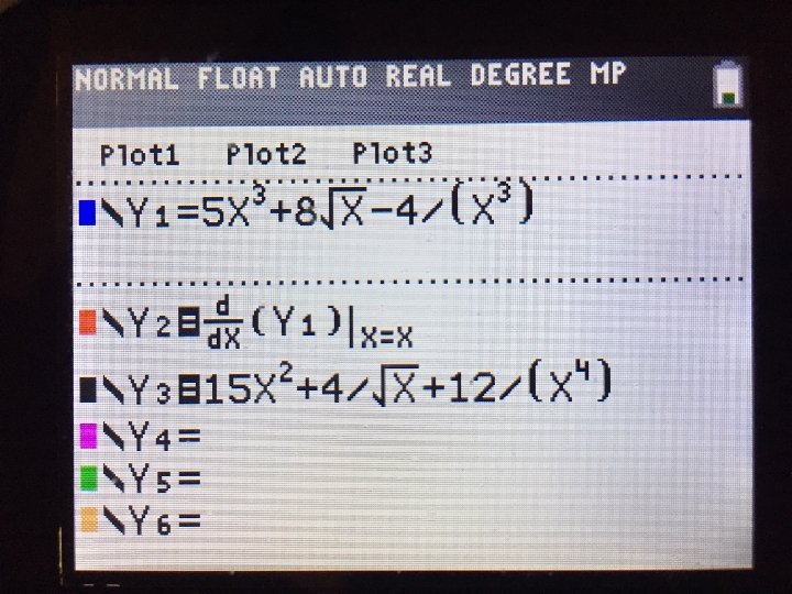
Hit the “zoom” button, scroll down, and choose “Zoom. Fit” in order to choose appropriate scales for your axes. Graph your functions. Use the “trace” button to trace along your graph. Toggle back and forth between tracing along Y 2 and Y 3. If you did the problem correctly, they will be the same graph.

Sine curves We’re all set for polynomials! Lots of phenomena in physics are cyclical, which means they are well represented by sine curves. What’s the derivative of sin x? Let’s approach this question graphically…

Let f(x) = sin x

Let f(x) = sin x Let’s draw tangent lines to the graph at the points where x = 0, 0. 5π, π, 1. 5π, and 2π

Let f(x) = sin x m m = = 1 m=0 -1 m=0 Careful analysis shows: when x = 0, slope = 1; when x = 0. 5π, slope = 0; when x = π, slope = -1; when x = 1. 5π, slope = 0, and when x = 2π, slope = 1.

So what function passes through the points (0, 1), (0. 5π, 0), (π, -1), (1. 5π, 0), and (2π, 1)? The answer: cos x

So what function passes through the points (0, 1), (0. 5π, 0), (π, -1), (1. 5π, 0), and (2π, 1)? The answer: cos x We’ve just demonstrated graphically that if f(x) = sin x, then f ‘(x) = cos x. A similar graphical approach can show that if f(x) = cos x, then f ‘(x) = - sin x.

Antidifferentiaion Let’s turn things around. Suppose you’re given f ’(x) = 20 x 3 – 6 x and asked to find a corresponding function f(x). In other words, you’re asked to find an antiderivative. Consider exponents first. When differentiating, exponents always decrease by 1, so going backwards, the exponents must increase by 1. Therefore, your antiderivative will be of the form f(x) = __x 4 - ___x 2 where the blanks are coefficients. To find the coefficients, imagine taking the derivative of f(x) and ask yourself, “What do you multiply by 4 to get 20? ” and “What do you multiply by 2 to get 6? ” Thus f(x) = 5 x 4 – 3 x 2 is an antiderivative of f ’(x) = 20 x 3 – 6 x

Note: I was careful to call f(x) = 5 x 4 – 3 x 2 an antiderivative of f ’(x) = 20 x 3 – 6 x and not the antiderivative. You could add or subtract any constant to f(x) and not change what its derivative would be since the derivative of any constant is zero. If you took the derivative of 5 x 4 – 3 x 2 + 7 or 5 x 4 – 3 x 2 – 42 or 5 x 4 – 3 x 2 + 1, 701, you’d get the same result: 20 x 3 – 6 x. This make sense when you think about it graphically. Adding or subtracting a constant just shifts a graph vertically on the x-y plane, but doesn’t change the value of the slope at any point.

Don’t forget the “+ c”!!! Therefore, if we want to be as generic as possible when asked to find the antiderivative of f ’(x) = 20 x 3 – 6 x we would say the answer is f(x) = 5 x 4 – 3 x 2 + c, where c is a constant. f(x) = 5 x 4 – 3 x 2 + c is said to be the “general antiderivative” of f ’(x) = 20 x 3 – 6 x. In the absence of any other information or instructions, always include “+ c” whenever you find an antiderivative!

Indefinite Integration The act of finding a function’s antiderivative is called “integration”, specifically “indefinite integration”. (We’ll get to “definite integration” soon…. ) Here are three ways to ask the same thing: f ’(x) = 20 x 3 – 6 x. Find f(x). Find the integral of 20 x 3 – 6 x. Evaluate:

Anatomy of an Indefinite Integral The integral sign – It lets you know that you’ll be taking an antiderivative The “integrand” – the function that you will be finding the antiderivative of This part just lets you know that the variable we’re working with is x. At this point it is helpful to think of the “dx” as punctuation, like the period at the end of the integral’s sentence.

Example Problem Evaluate the following integral such that the result passes through the point (2, 5).

Solution We know that when x = 2, y = 5, so we can say: So, the final answer is:

Back to the Area Problem So what does all this have to do with the other big problem of calculus – the area problem? And what is a “definite integral”? We’re almost there! To get there, let’s revisit the related concepts of velocity, distance, and time. Recall: Velocity is the derivative of a position v. time curve.

Revisiting Velocity, Distance and Time Velocity is defined as a change in position divided by the time it took to change position: Solving for change in position yields: Note: This only works if velocity is constant during the interval Δt. Let’s consider this graphically…

constant, change in position is given by Δx = v Δt Graphically, this calculation represents the area of the rectangle beneath the vel. vs time curve. What if velocity isn’t constant? velocity (m/s) When velocity is Time (s)

where velocity varies directly with time. Change in position can still be calculated by finding the area under the curve. In the case the region is a trapezoid, whose area is given by a simple formula from geometry. velocity (m/s) Consider a situation Time (s)

situation where velocity varies with time in a nonlinear fashion. (Forgive me if this seems a jerk move. ) How do we calculate the area under a curve like this? velocity (m/s) Now let’s consider a Recall that velocity is the derivative of a position function. Therefore, position must be the antiderivative of the velocity function! Time (s) To calculate the area under a curve, we will use a “definite integral” and the Fundamental Theorem of Calculus

The Fundamental Theorem of Calculus The area between the graphs of f(x) the x-axis and between the values of x = a and x = b is given by: where F(x) is the antiderivative of f(x), and a and b are the “lower limit of integration” and “upper limit of integration” respectively.

Example Problem Find the area of the region bounded by the graphs of y = √x, the x-axis, and the vertical lines x = 1 and x = 9.

Set up the definite integral: Rewrite integrand: Find the antiderivative: (Note: the “+c” isn’t needed here) Evaluate the antiderivative at the upper and lower limits of integration and subtract:

Checking your answer Once again you can check your answer using your graphing calculator. If you have a TI grapher, hit the “math” button and choose “fnint(“

Or, if you want to check your answer in more graphical (and in my opinion, spiffier) way: Hit the “y=“ button and enter the function you’re finding the area under as Y 1. (Make sure you’re zoomed such that your axes have appropriate upper and lower limits. ) Hit the “ 2 nd” and “trace” buttons for the “calc” menu. The choose the integration option. Input the lower and upper limits of integration. The region you’re find the area of will get shaded in and the answer will appear on the screen.

A few things to consider… Any area that occurs beneath the x-axis is considered negative. With this in mind, what’s the best way to approach this problem? Evaluate the integral:

One could go through the steps of find the antiderivative and evaluating it at the upper and lower limits of integration, and they would get the correct answer. However let’s look at the graph: One can reason that the area above the xaxis from 0 to π is equal to the area below the x-axis from π to 2π. Since the area below the x-axis is considered negative, you can conclude the total answer is 0.

Your Goal In this class your goal is not simply to determine the right answer to a question. Your goal should be to find the most efficient path to that answer! Sometimes a problem that would take a long time using calculus (or perhaps couldn’t even be done using calculus!) can be done very quickly using a little geometry or simple reasoning, as was the case in the previous example. Since the AP exam is a timed exam, you will want to be well-practiced at finding the most expeditious way of doing problems!