Calculator steps n The calculator steps for this

Calculator steps: n The calculator steps for this section can be found on You. Tube or by clicking: Here Bluman, Chapter 11 1

While you wait for class to start: 1. I. II. 2. Please create two lists on your calculator name them: OBS… short for observed EXP… short for expected Find the GOF test on your calculator Bluman, Chapter 11 2

Chapter 11 Other Chi-Square Tests Mc. Graw-Hill, Bluman, 7 th ed. , Chapter 11 3

Chapter 11 Overview n Introduction 11 -1 Test for Goodness of Fit n 11 -2 Tests Using Contingency Tables Bluman, Chapter 11 4

Chapter 11 Objectives 1. Test a distribution for goodness of fit, using chi -square. 2. Test two variables for independence, using chi -square. 3. Test proportions for homogeneity, using chi-square. Bluman, Chapter 11 5

11. 1 Test for Goodness of Fit n The chi-square statistic can be used to see whether a frequency distribution fits a specific pattern. This is referred to as the chi-square goodness-of-fit test. Bluman, Chapter 11 6

Test for Goodness of Fit Formula for the test for goodness of fit: where d. f. = number of categories minus 1 O = observed frequency E = expected frequency Bluman, Chapter 11 7

Assumptions for Goodness of Fit 1. The data are obtained from a random sample. 2. The expected frequency for each category must be 5 or more. Bluman, Chapter 11 8

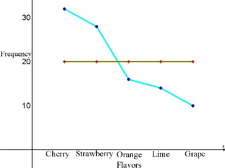
Observed vs. Expected Graph o To get some idea of why this test is called the goodness-of-fit test, examine graphs of the observed values and expected values. From the graphs, one can see whether the observed values and expected values are close together or far apart.

Assumptions Based on Graphs When the observed values and expected values are close together, the chi-square test value will be small. o Then the decision will be to not reject the null hypothesis—hence , there is “a good fit. ” o

Assumptions Based on Graphs o When the observed values and the expected values are far apart, the chi-square test value will be large. o Then, the null hypothesis will be rejected—hence, there is “not a good fit. ”

Page 595

Chapter 11 Other Chi-Square Tests Section 11 -1 Example 11 -1 Page #592 Bluman, Chapter 11 14

Example 11 -1: Fruit Soda Flavors A market analyst wished to see whether consumers have any preference among five flavors of a new fruit soda. A sample of 100 people provided the following data. Is there enough evidence to reject the claim that there is no preference in the selection of fruit soda flavors, using the data shown previously? Let α = 0. 05. Cherry Strawberry Orange Lime Grape Observed 32 28 16 14 10 Expected 20 20 20 Step 1: State the hypotheses and identify the claim. H 0: Consumers show no preference (claim). H 1: Consumers show a preference. Bluman, Chapter 11 15

Example 11 -1: Fruit Soda Flavors Cherry Strawberry Orange Lime Grape Observed 32 28 16 14 10 Expected 20 20 20 Step 2: Find the critical value. D. f. = 5 – 1 = 4, and α = 0. 05. CV = 9. 488. Step 3: Compute the test value. Bluman, Chapter 11 16

Example 11 -1: Fruit Soda Flavors Step 4: Make the decision. The decision is to reject the null hypothesis, since 18. 0 > 9. 488. Step 5: Summarize the results. There is enough evidence to reject the claim that consumers show no preference for the flavors. Bluman, Chapter 11 17

Enter expected and observed values: Df= number of catagories-1 Bluman, Chapter 11

Chapter 11 Other Chi-Square Tests Section 11 -1 Example 11 -2 Page #594 Bluman, Chapter 11 19

Example 11 -2: Retirees The Russel Reynold Association surveyed retired senior executives who had returned to work. They found that after returning to work, 38% were employed by another organization, 32% were self-employed, 23% were either freelancing or consulting, and 7% had formed their own companies. To see if these percentages are consistent with those of Allegheny County residents, a local researcher surveyed 300 retired executives who had returned to work and found that 122 were working for another company, 85 were self-employed, 76 were either freelancing or consulting, and 17 had formed their own companies. At α = 0. 10, test the claim that the percentages are the same for those people in Allegheny County. Bluman, Chapter 11 20

Example 11 -2: Retirees New Company Self. Employed Freelancing Owns Company Observed 122 85 76 17 Expected . 38(300)= 114 . 32(300)= 96 . 23(300)= 69 . 07(300)= 21 Step 1: State the hypotheses and identify the claim. H 0: The retired executives who returned to work are distributed as follows: 38% are employed by another organization, 32% are selfemployed, 23% are either freelancing or consulting, and 7% have formed their own companies (claim). H 1: The distribution is not the same as stated in the null hypothesis. Bluman, Chapter 11 21

Input the observed values: Input the expected: Calculate as you enter the values: The method above produces the most accurate result and it saves time. Bluman, Chapter 11 22

Notice: the df is 3, which is one less than the number of categories. Bluman, Chapter 11 23

Example 11 -2: Retirees New Company Self. Employed Freelancing Owns Company Observed 122 85 76 17 Expected . 38(300)= 114 . 32(300)= 96 . 23(300)= 69 . 07(300)= 21 Step 2: Find the critical value. D. f. = 4 – 1 = 3, and α = 0. 10. CV = 6. 251. Step 3: Compute the test value. Bluman, Chapter 11 24

Example 11 -2: Retirees Step 4: Make the decision. Since 3. 2939 < 6. 251, the decision is not to reject the null hypothesis. Step 5: Summarize the results. There is not enough evidence to reject the claim. It can be concluded that the percentages are not significantly different from those given in the null hypothesis. Bluman, Chapter 11 25

Chapter 11 Other Chi-Square Tests Section 11 -1 Example 11 -3 Page #595 Bluman, Chapter 11 26

Example 11 -3: Firearm Deaths A researcher read that firearm-related deaths for people aged 1 to 18 were distributed as follows: 74% were accidental, 16% were homicides, and 10% were suicides. In her district, there were 68 accidental deaths, 27 homicides, and 5 suicides during the past year. At α= 0. 10, test the claim that the percentages are equal. Accidental Homicides Suicides Observed 68 27 5 Expected 74 16 10 Bluman, Chapter 11 27

Example 11 -3: Firearm Deaths Accidental Homicides Suicides Observed 68 27 5 Expected 74 16 10 Step 1: State the hypotheses and identify the claim. H 0: Deaths due to firearms for people aged 1 through 18 are distributed as follows: 74% accidental, 16% homicides, and 10% suicides (claim). H 1: The distribution is not the same as stated in the null hypothesis. Bluman, Chapter 11 28

Example 11 -3: Firearm Deaths Accidental Homicides Suicides Observed 68 27 5 Expected 74 16 10 Step 2: Find the critical value. D. f. = 3 – 1 = 2, and α = 0. 10. CV = 4. 605. Step 3: Compute the test value. Bluman, Chapter 11 29

Example 11 -3: Firearm Deaths Step 4: Make the decision. Reject the null hypothesis, since 10. 549 > 4. 605. Step 5: Summarize the results. There is enough evidence to reject the claim that the distribution is 74% accidental, 16% homicides, and 10% suicides. Bluman, Chapter 11 30

Test for Normality (Optional) n n n The chi-square goodness-of-fit test can be used to test a variable to see if it is normally distributed. The hypotheses are: ¨ H 0: The variable is normally distributed. ¨ H 1: The variable is not normally distributed. This procedure is somewhat complicated. The calculations are shown in example 11 -4 on page 597 in the text. Bluman, Chapter 11 31

On your own n Read section 11. 1 n n n Homework: Sec 11. 1 page 601 #1 -4 all #5, 11, 13 Bluman, Chapter 11 32