Cache Memories Topics n n Generic cache memory




- Slides: 39

Cache Memories Topics n n Generic cache memory organization Direct mapped caches Set associative caches Impact of caches on performance

Cache Memories Cache memories are small, fast SRAM-based memories managed automatically in hardware. n Hold frequently accessed blocks of main memory CPU looks first for data in L 1, then in L 2, then in main memory. Typical bus structure: CPU chip register file cache bus L 2 cache – 2– L 1 cache bus interface ALU system bus memory bus I/O bridge main memory

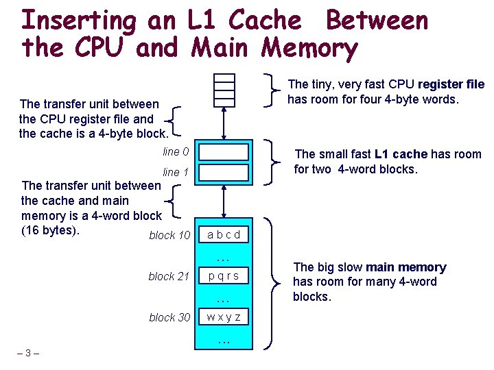
Inserting an L 1 Cache Between the CPU and Main Memory The tiny, very fast CPU register file has room for four 4 -byte words. The transfer unit between the CPU register file and the cache is a 4 -byte block. line 0 The small fast L 1 cache has room for two 4 -word blocks. line 1 The transfer unit between the cache and main memory is a 4 -word block (16 bytes). block 10 abcd . . . block 21 pqrs . . . block 30 wxyz . . . – 3– The big slow main memory has room for many 4 -word blocks.

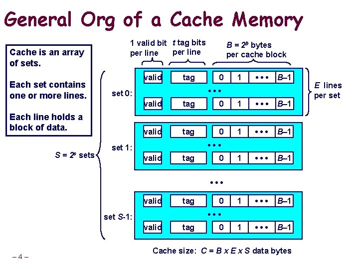
General Org of a Cache Memory Cache is an array of sets. Each set contains one or more lines. 1 valid bit t tag bits per line valid S= 0 1 • • • B– 1 • • • set 0: Each line holds a block of data. 2 s sets tag B = 2 b bytes per cache block valid tag 0 1 • • • B– 1 1 • • • B– 1 • • • set 1: valid tag 0 • • • valid tag • • • set S-1: valid – 4– 0 tag 0 Cache size: C = B x E x S data bytes E lines per set

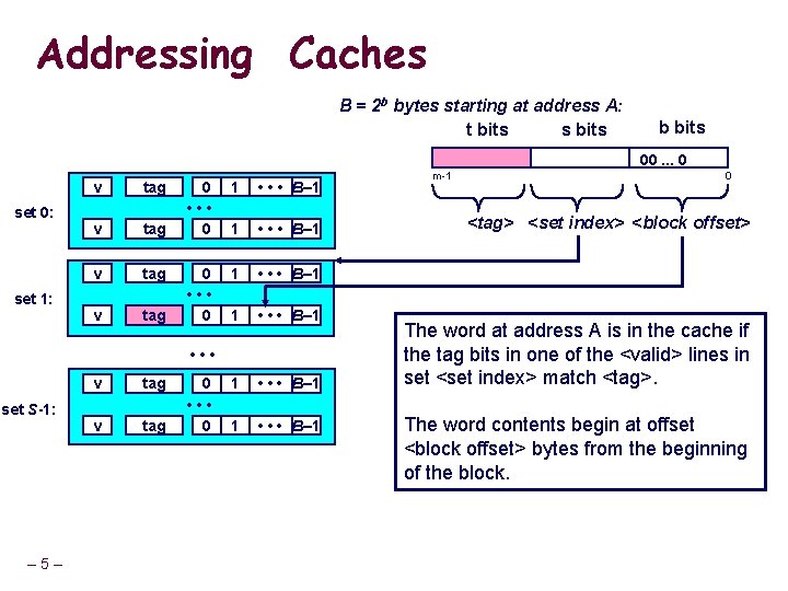
Addressing Caches B = 2 b bytes starting at address A: t bits s bits b bits 00. . . 0 set 0: set 1: v tag 0 • • • 0 1 • • • B– 1 1 • • • B– 1 • • • set S-1: – 5– v tag 0 • • • 0 m-1 0 <tag> <set index> <block offset> The word at address A is in the cache if the tag bits in one of the <valid> lines in set <set index> match <tag>. The word contents begin at offset <block offset> bytes from the beginning of the block.

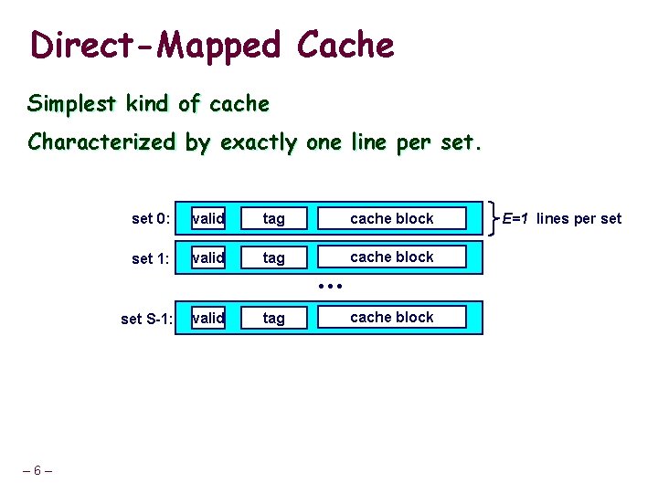
Direct-Mapped Cache Simplest kind of cache Characterized by exactly one line per set 0: valid tag cache block set 1: valid tag cache block • • • set S-1: – 6– valid tag cache block E=1 lines per set

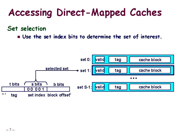
Accessing Direct-Mapped Caches Set selection n Use the set index bits to determine the set of interest. selected set 0: valid tag cache block set 1: valid tag cache block • • • t bits m-1 tag – 7– s bits b bits 0 0 1 set index block offset 0 set S-1: valid tag cache block

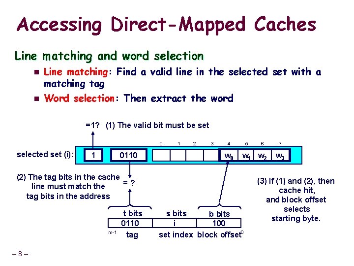
Accessing Direct-Mapped Caches Line matching and word selection n n Line matching: Find a valid line in the selected set with a matching tag Word selection: Then extract the word =1? (1) The valid bit must be set 0 selected set (i): 1 0110 1 2 3 4 w 0 5 w 1 w 2 (2) The tag bits in the cache = ? line must match the tag bits in the address m-1 – 8– t bits 0110 tag 6 s bits b bits i 100 set index block offset 0 7 w 3 (3) If (1) and (2), then cache hit, and block offset selects starting byte.

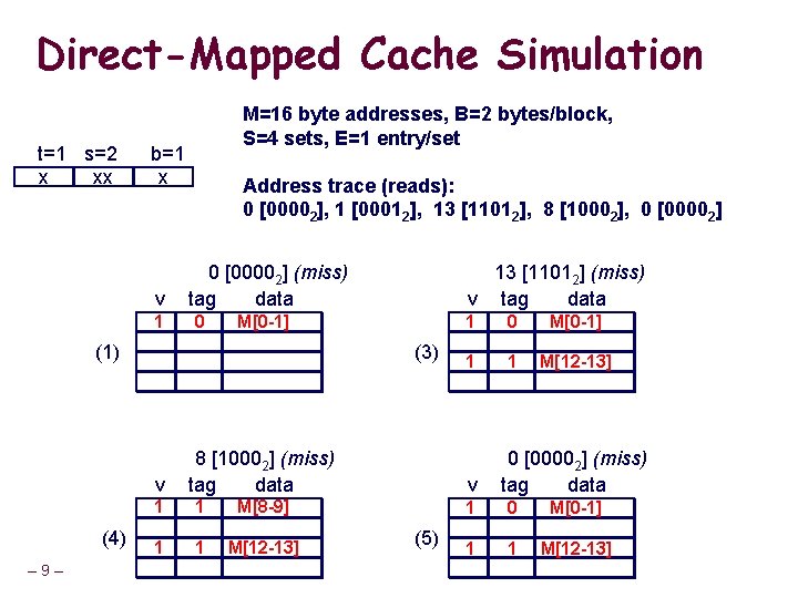
Direct-Mapped Cache Simulation t=1 s=2 x xx M=16 byte addresses, B=2 bytes/block, S=4 sets, E=1 entry/set b=1 x v 11 Address trace (reads): 0 [00002], 1 [00012], 13 [11012], 8 [10002], 0 [00002] (miss) tag data 0 m[1] m[0] M[0 -1] (1) (3) v (4) – 9– 13 [11012] (miss) v tag data 8 [10002] (miss) tag data 11 1 m[9] m[8] M[8 -9] 1 1 M[12 -13] 1 1 0 m[1] m[0] M[0 -1] 1 1 1 m[13] m[12] M[12 -13] v (5) 0 [00002] (miss) tag data 11 0 m[1] m[0] M[0 -1] 11 1 m[13] m[12] M[12 -13]

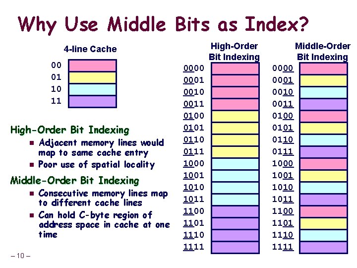
Why Use Middle Bits as Index? High-Order Bit Indexing 4 -line Cache 00 01 10 11 High-Order Bit Indexing n n Adjacent memory lines would map to same cache entry Poor use of spatial locality Middle-Order Bit Indexing n n – 10 – Consecutive memory lines map to different cache lines Can hold C-byte region of address space in cache at one time 0000 0001 0010 0011 0100 0101 0110 0111 1000 1001 1010 1011 1100 1101 1110 1111 Middle-Order Bit Indexing 0000 0001 0010 0011 0100 0101 0110 0111 1000 1001 1010 1011 1100 1101 1110 1111

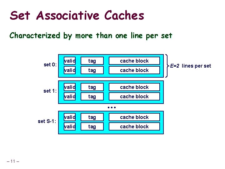
Set Associative Caches Characterized by more than one line per set 0: set 1: valid tag cache block • • • set S-1: – 11 – valid tag cache block E=2 lines per set

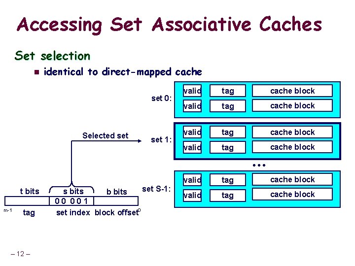
Accessing Set Associative Caches Set selection n identical to direct-mapped cache set 0: Selected set 1: valid tag cache block • • • t bits m-1 tag – 12 – set S-1: s bits b bits 0 0 1 set index block offset 0 valid tag cache block

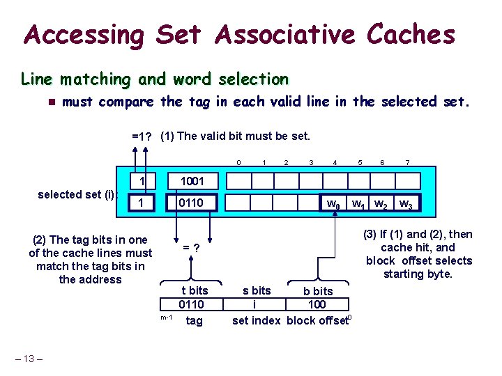
Accessing Set Associative Caches Line matching and word selection n must compare the tag in each valid line in the selected set. =1? (1) The valid bit must be set. 0 selected set (i): 1 1001 1 0110 (2) The tag bits in one of the cache lines must match the tag bits in the address 2 3 4 w 0 t bits 0110 tag 5 6 w 1 w 2 7 w 3 (3) If (1) and (2), then cache hit, and block offset selects starting byte. = ? m-1 – 13 – 1 s bits b bits i 100 set index block offset 0

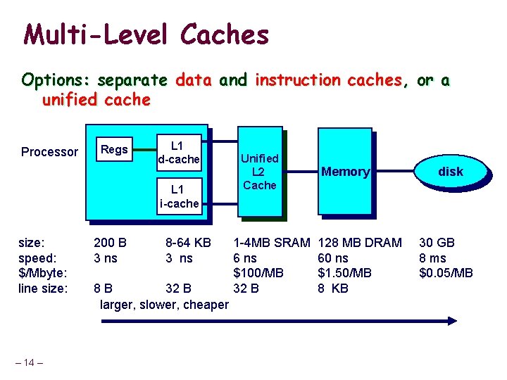
Multi-Level Caches Options: separate data and instruction caches, or a unified cache Processor Regs L 1 d-cache L 1 i-cache size: speed: $/Mbyte: line size: – 14 – 200 B 3 ns 8 -64 KB 3 ns 8 B 32 B larger, slower, cheaper Unified L 2 Cache 1 -4 MB SRAM 6 ns $100/MB 32 B Memory 128 MB DRAM 60 ns $1. 50/MB 8 KB disk 30 GB 8 ms $0. 05/MB

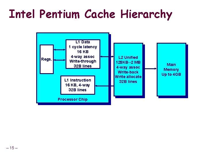
Intel Pentium Cache Hierarchy Regs. L 1 Data 1 cycle latency 16 KB 4 -way assoc Write-through 32 B lines L 1 Instruction 16 KB, 4 -way 32 B lines Processor Chip – 15 – L 2 Unified 128 KB--2 MB 4 -way assoc Write-back Write allocate 32 B lines Main Memory Up to 4 GB

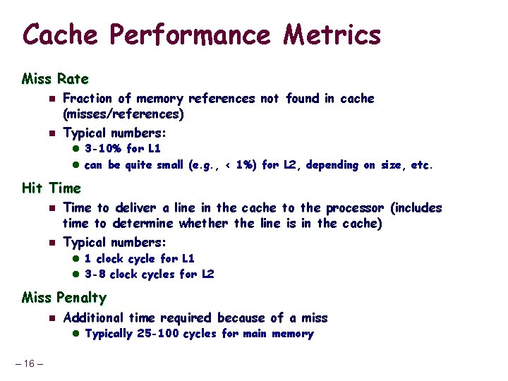
Cache Performance Metrics Miss Rate n n Fraction of memory references not found in cache (misses/references) Typical numbers: l 3 -10% for L 1 l can be quite small (e. g. , < 1%) for L 2, depending on size, etc. Hit Time n n Time to deliver a line in the cache to the processor (includes time to determine whether the line is in the cache) Typical numbers: l 1 clock cycle for L 1 l 3 -8 clock cycles for L 2 Miss Penalty n Additional time required because of a miss l Typically 25 -100 cycles for main memory – 16 –

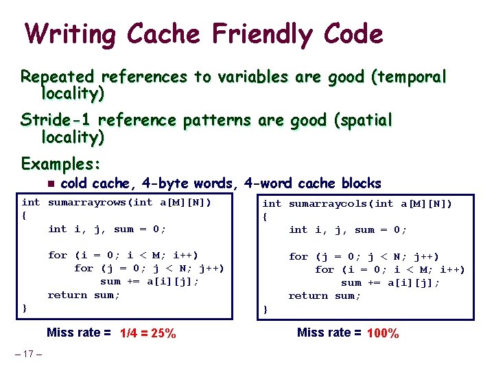
Writing Cache Friendly Code Repeated references to variables are good (temporal locality) Stride-1 reference patterns are good (spatial locality) Examples: n cold cache, 4 -byte words, 4 -word cache blocks int sumarrayrows(int a[M][N]) { int i, j, sum = 0; int sumarraycols(int a[M][N]) { int i, j, sum = 0; for (i = 0; i < M; i++) for (j = 0; j < N; j++) sum += a[i][j]; return sum; } } Miss rate = 1/4 = 25% – 17 – for (j = 0; j < N; j++) for (i = 0; i < M; i++) sum += a[i][j]; return sum; Miss rate = 100%

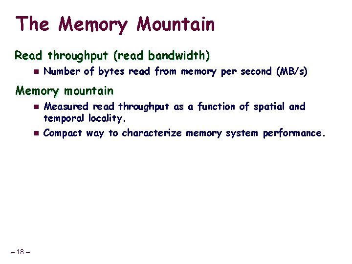
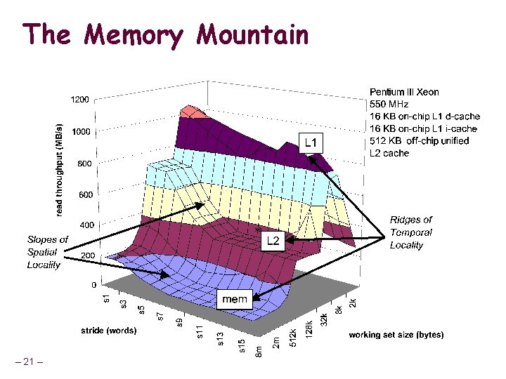
The Memory Mountain Read throughput (read bandwidth) n Number of bytes read from memory per second (MB/s) Memory mountain n n – 18 – Measured read throughput as a function of spatial and temporal locality. Compact way to characterize memory system performance.

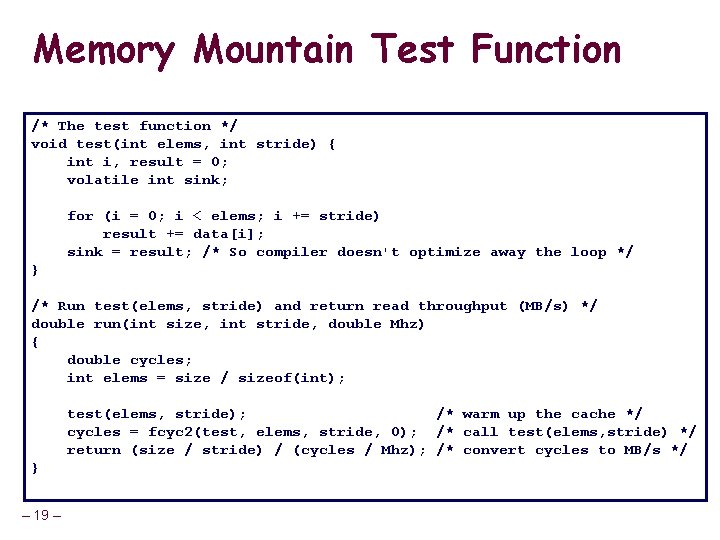
Memory Mountain Test Function /* The test function */ void test(int elems, int stride) { int i, result = 0; volatile int sink; for (i = 0; i < elems; i += stride) result += data[i]; sink = result; /* So compiler doesn't optimize away the loop */ } /* Run test(elems, stride) and return read throughput (MB/s) */ double run(int size, int stride, double Mhz) { double cycles; int elems = size / sizeof(int); test(elems, stride); /* warm up the cache */ cycles = fcyc 2(test, elems, stride, 0); /* call test(elems, stride) */ return (size / stride) / (cycles / Mhz); /* convert cycles to MB/s */ } – 19 –

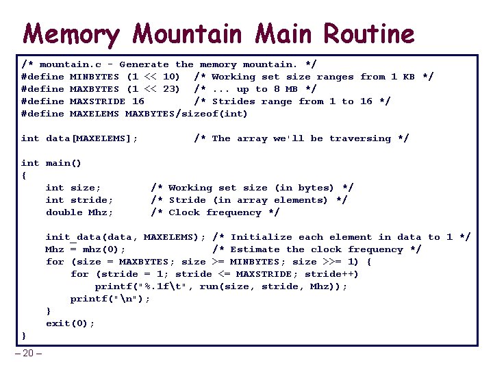
Memory Mountain Main Routine /* mountain. c - Generate the memory mountain. */ #define MINBYTES (1 << 10) /* Working set size ranges from 1 KB */ #define MAXBYTES (1 << 23) /*. . . up to 8 MB */ #define MAXSTRIDE 16 /* Strides range from 1 to 16 */ #define MAXELEMS MAXBYTES/sizeof(int) int data[MAXELEMS]; int main() { int size; int stride; double Mhz; /* The array we'll be traversing */ /* Working set size (in bytes) */ /* Stride (in array elements) */ /* Clock frequency */ init_data(data, MAXELEMS); /* Initialize each element in data to 1 */ Mhz = mhz(0); /* Estimate the clock frequency */ for (size = MAXBYTES; size >= MINBYTES; size >>= 1) { for (stride = 1; stride <= MAXSTRIDE; stride++) printf("%. 1 ft", run(size, stride, Mhz)); printf("n"); } exit(0); } – 20 –

The Memory Mountain – 21 –

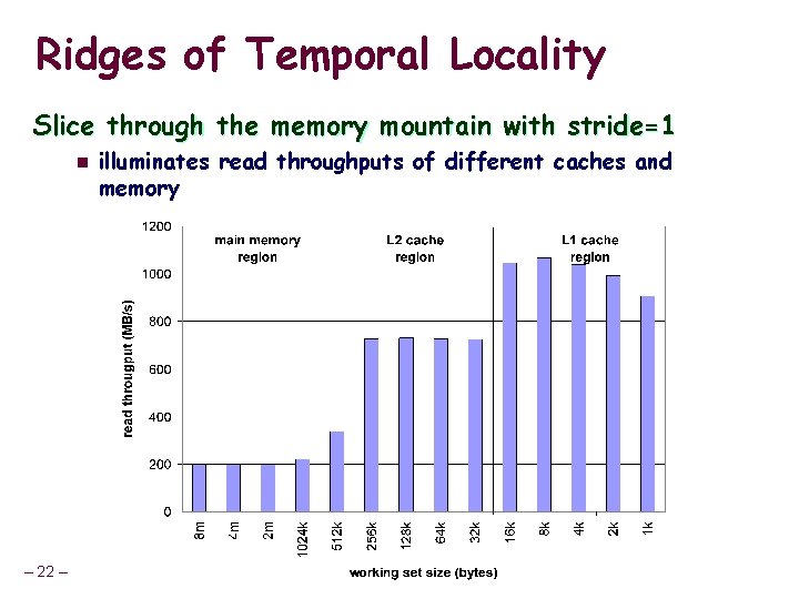
Ridges of Temporal Locality Slice through the memory mountain with stride=1 n – 22 – illuminates read throughputs of different caches and memory

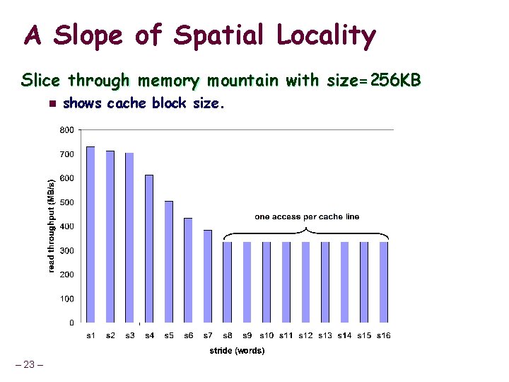
A Slope of Spatial Locality Slice through memory mountain with size=256 KB n – 23 – shows cache block size.

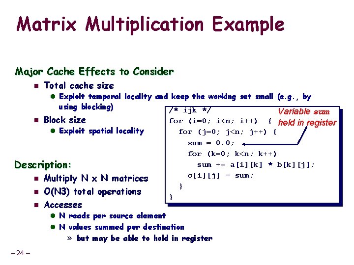
Matrix Multiplication Example Major Cache Effects to Consider n Total cache size l Exploit temporal locality and keep the working set small (e. g. , by using blocking) n Block size l Exploit spatial locality Description: n n n Multiply N x N matrices O(N 3) total operations Accesses /* ijk */ Variable sum for (i=0; i<n; i++) { held in register for (j=0; j<n; j++) { sum = 0. 0; for (k=0; k<n; k++) sum += a[i][k] * b[k][j]; c[i][j] = sum; } } l N reads per source element l N values summed per destination » but may be able to hold in register – 24 –

Miss Rate Analysis for Matrix Multiply Assume: n n Line size = 32 B (big enough for 4 64 -bit words) Matrix dimension (N) is very large l Approximate 1/N as 0. 0 n Cache is not even big enough to hold multiple rows Analysis Method: n Look at access pattern of inner loop k i j k A – 25 – j i B C

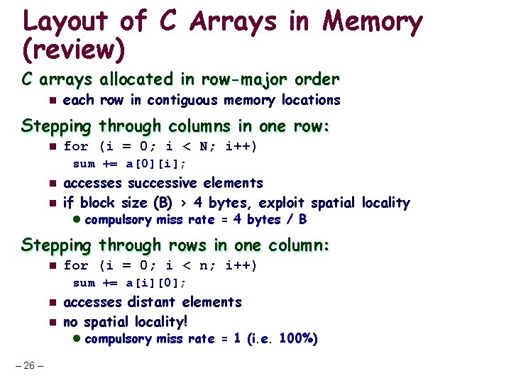
Layout of C Arrays in Memory (review) C arrays allocated in row-major order n each row in contiguous memory locations Stepping through columns in one row: n for (i = 0; i < N; i++) sum += a[0][i]; n n accesses successive elements if block size (B) > 4 bytes, exploit spatial locality l compulsory miss rate = 4 bytes / B Stepping through rows in one column: n for (i = 0; i < n; i++) sum += a[i][0]; n n accesses distant elements no spatial locality! l compulsory miss rate = 1 (i. e. 100%) – 26 –

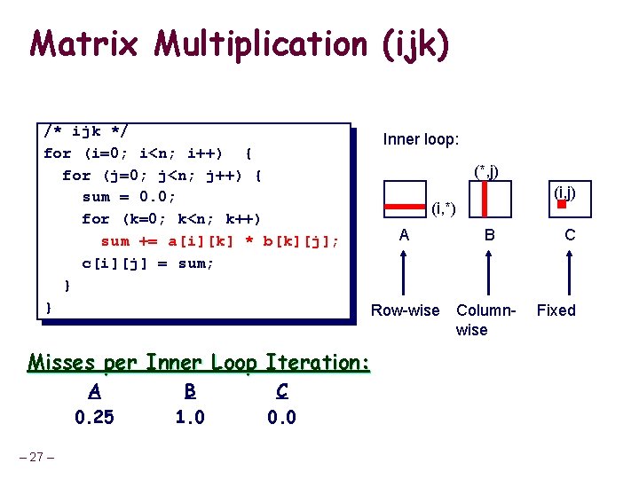
Matrix Multiplication (ijk) /* ijk */ for (i=0; i<n; i++) { for (j=0; j<n; j++) { sum = 0. 0; for (k=0; k<n; k++) sum += a[i][k] * b[k][j]; c[i][j] = sum; } } Misses per Inner Loop Iteration: A 0. 25 – 27 – B 1. 0 C 0. 0 Inner loop: (*, j) (i, *) A B Row-wise Columnwise C Fixed

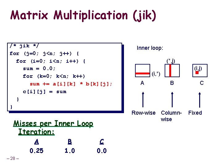
Matrix Multiplication (jik) /* jik */ for (j=0; j<n; j++) { for (i=0; i<n; i++) { sum = 0. 0; for (k=0; k<n; k++) sum += a[i][k] * b[k][j]; c[i][j] = sum } } Misses per Inner Loop Iteration: A 0. 25 – 28 – B 1. 0 C 0. 0 Inner loop: (*, j) (i, *) A B Row-wise Columnwise C Fixed

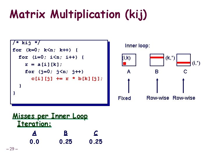
Matrix Multiplication (kij) /* kij */ for (k=0; k<n; k++) { for (i=0; i<n; i++) { r = a[i][k]; for (j=0; j<n; j++) c[i][j] += r * b[k][j]; } } Misses per Inner Loop Iteration: A 0. 0 – 29 – B 0. 25 C 0. 25 Inner loop: (i, k) A Fixed (k, *) B (i, *) C Row-wise

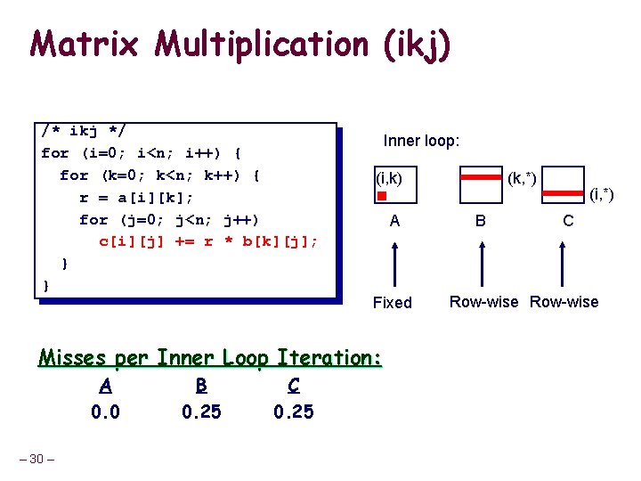
Matrix Multiplication (ikj) /* ikj */ for (i=0; i<n; i++) { for (k=0; k<n; k++) { r = a[i][k]; for (j=0; j<n; j++) c[i][j] += r * b[k][j]; } } Inner loop: (i, k) A Fixed Misses per Inner Loop Iteration: A 0. 0 – 30 – B 0. 25 C 0. 25 (k, *) B (i, *) C Row-wise

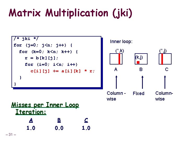
Matrix Multiplication (jki) /* jki */ for (j=0; j<n; j++) { for (k=0; k<n; k++) { r = b[k][j]; for (i=0; i<n; i++) c[i][j] += a[i][k] * r; } } – 31 – B 0. 0 (*, k) C 1. 0 (*, j) (k, j) A Column wise Misses per Inner Loop Iteration: A 1. 0 Inner loop: B Fixed C Columnwise

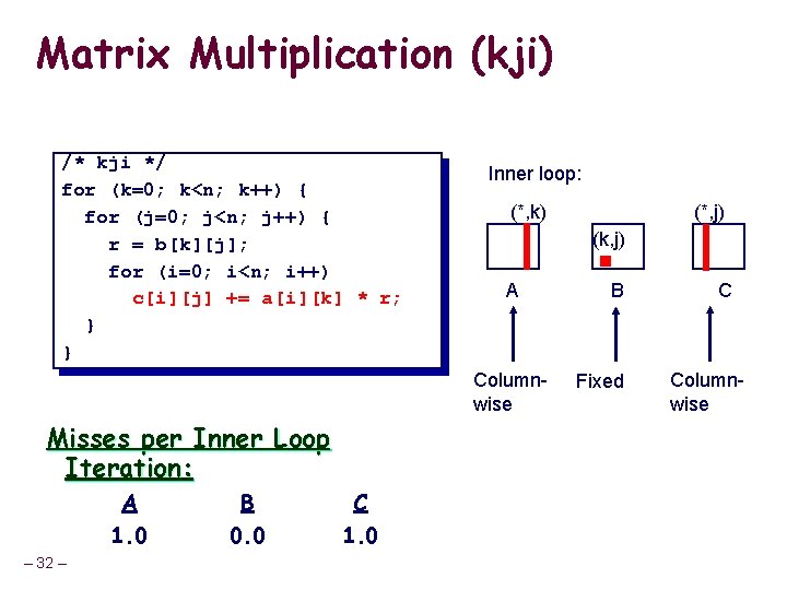
Matrix Multiplication (kji) /* kji */ for (k=0; k<n; k++) { for (j=0; j<n; j++) { r = b[k][j]; for (i=0; i<n; i++) c[i][j] += a[i][k] * r; } } Inner loop: (*, k) (k, j) A Columnwise Misses per Inner Loop Iteration: A 1. 0 – 32 – B 0. 0 C 1. 0 (*, j) B Fixed C Columnwise

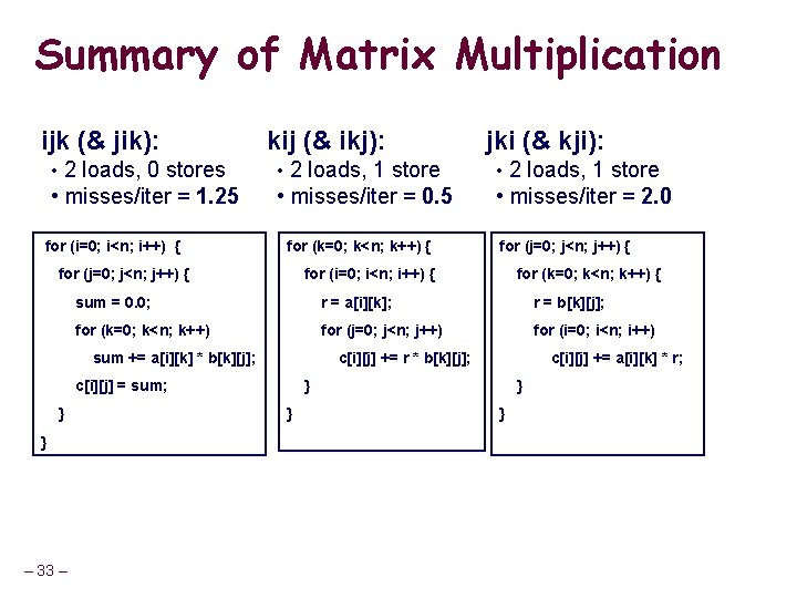
Summary of Matrix Multiplication ijk (& jik): kij (& ikj): jki (& kji): • 2 loads, 0 stores • 2 loads, 1 store • misses/iter = 1. 25 • misses/iter = 0. 5 • misses/iter = 2. 0 for (i=0; i<n; i++) { for (k=0; k<n; k++) { for (j=0; j<n; j++) { for (i=0; i<n; i++) { for (k=0; k<n; k++) { sum = 0. 0; r = a[i][k]; r = b[k][j]; for (k=0; k<n; k++) for (j=0; j<n; j++) for (i=0; i<n; i++) sum += a[i][k] * b[k][j]; c[i][j] += r * b[k][j]; c[i][j] += a[i][k] * r; c[i][j] = sum; } } } – 33 –

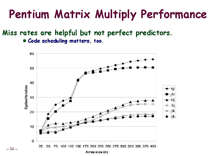
Pentium Matrix Multiply Performance Miss rates are helpful but not perfect predictors. l Code scheduling matters, too. – 34 –

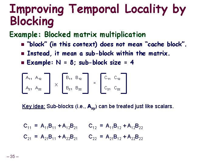
Improving Temporal Locality by Blocking Example: Blocked matrix multiplication n “block” (in this context) does not mean “cache block”. Instead, it mean a sub-block within the matrix. Example: N = 8; sub-block size = 4 A 11 A 12 A 21 A 22 B 11 B 12 X B 21 B 22 = C 11 C 12 C 21 C 22 Key idea: Sub-blocks (i. e. , Axy) can be treated just like scalars. – 35 – C 11 = A 11 B 11 + A 12 B 21 C 12 = A 11 B 12 + A 12 B 22 C 21 = A 21 B 11 + A 22 B 21 C 22 = A 21 B 12 + A 22 B 22

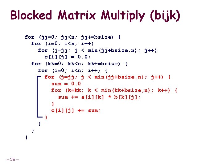
Blocked Matrix Multiply (bijk) for (jj=0; jj<n; jj+=bsize) { for (i=0; i<n; i++) for (j=jj; j < min(jj+bsize, n); j++) c[i][j] = 0. 0; for (kk=0; kk<n; kk+=bsize) { for (i=0; i<n; i++) { for (j=jj; j < min(jj+bsize, n); j++) { sum = 0. 0 for (k=kk; k < min(kk+bsize, n); k++) { sum += a[i][k] * b[k][j]; } c[i][j] += sum; } } – 36 –

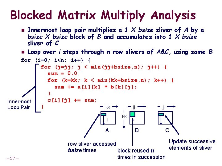
Blocked Matrix Multiply Analysis n n Innermost loop pair multiplies a 1 X bsize sliver of A by a bsize X bsize block of B and accumulates into 1 X bsize sliver of C Loop over i steps through n row slivers of A&C, using same B for (i=0; i<n; i++) { for (j=jj; j < min(jj+bsize, n); j++) { sum = 0. 0 for (k=kk; k < min(kk+bsize, n); k++) { sum += a[i][k] * b[k][j]; } c[i][j] += sum; Innermost } kk jj jj Loop Pair i A – 37 – kk i B C Update successive row sliver accessed elements of sliver bsize times block reused n times in succession

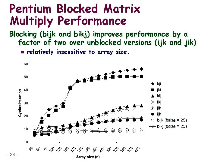
Pentium Blocked Matrix Multiply Performance Blocking (bijk and bikj) improves performance by a factor of two over unblocked versions (ijk and jik) n – 38 – relatively insensitive to array size.

Concluding Observations Programmer can optimize for cache performance n n How data structures are organized How data are accessed l Nested loop structure l Blocking is a general technique All systems favor “cache friendly code” n Getting absolute optimum performance is very platform specific l Cache sizes, line sizes, associativities, etc. n Can get most of the advantage with generic code l Keep working set reasonably small (temporal locality) l Use small strides (spatial locality) – 39 –