C Data Structures Introduction to Time Complexities 1

C++ Data Structures Introduction to Time Complexities 1

Algorithm Behavior • If an algorithm works with varying amounts of data each time it runs, we would normally expect that • When working with a large amount of data (in an array, for example), the algorithm would take longer to complete execution • When working with a small amount of data, the algorithm would complete execution more quickly 2

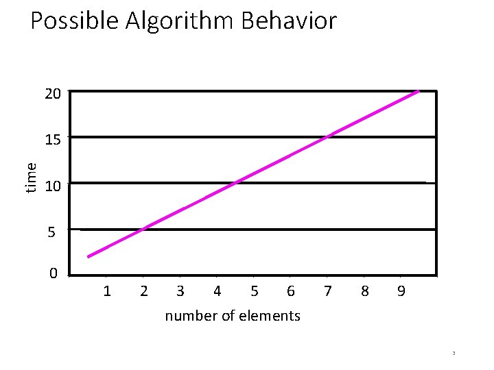
Possible Algorithm Behavior 20 time 15 10 5 0 1 2 3 4 5 6 number of elements 7 8 9 3

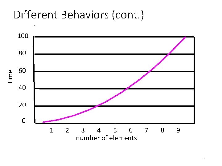
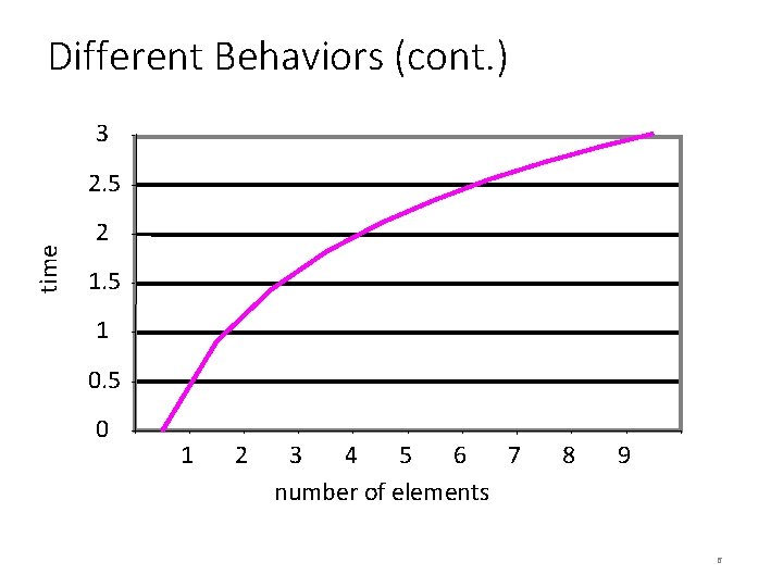
Different Behaviors • However, an algorithm’s behavior, as the number of elements is varied, does not always produce a nice straight line… 4

Different Behaviors (cont. ) 100 time 80 60 40 20 0 1 2 3 4 5 6 number of elements 7 8 9 5

Different Behaviors (cont. ) 3 time 2. 5 2 1. 5 1 0. 5 0 1 2 3 4 5 6 7 number of elements 8 9 6

Time Complexities • The different behaviors that you see actually represent different time complexities • Time complexities are used to help make an intelligent decision about which algorithm to use, when two different algorithms accomplish the same task 7

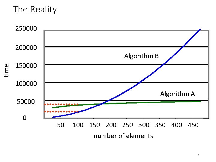
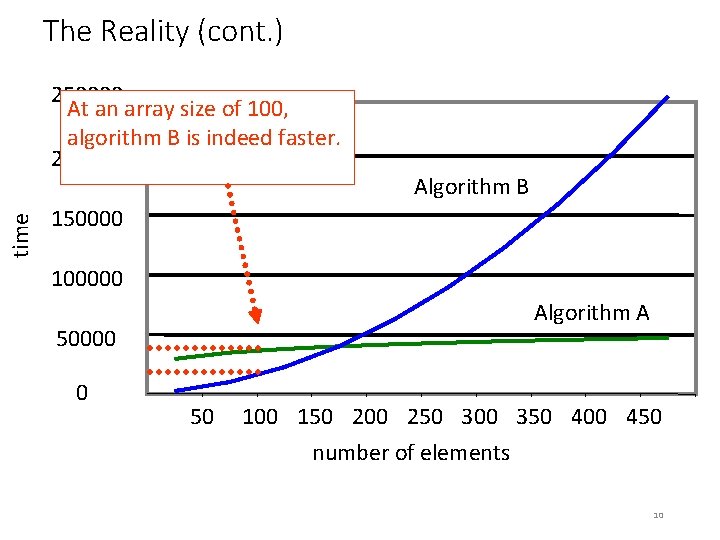
An Example • A decision needs to be made about which algorithm to use, algorithm A or algorithm B • They both accomplish the same task, but they use radically different methods to achieve the same result • One mountain top, but many ways up • They are timed, using millions of trials automated on a computer, and an array size of 100 • Algorithm B turned out to be faster. 8

The Reality 250000 time 200000 Algorithm B 150000 100000 Algorithm A 50000 0 50 100 150 200 250 300 350 400 450 number of elements 9

The Reality (cont. ) time 250000 At an array size of 100, algorithm B is indeed faster. 200000 Algorithm B 150000 100000 Algorithm A 50000 0 50 100 150 200 250 300 350 400 450 number of elements 10

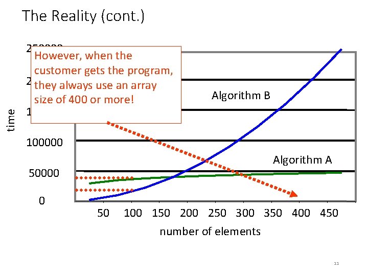
time The Reality (cont. ) 250000 However, when the customer gets the program, 200000 they always use an array size of 400 or more! 150000 Algorithm B 100000 Algorithm A 50000 0 50 100 150 200 250 300 350 400 450 number of elements 11

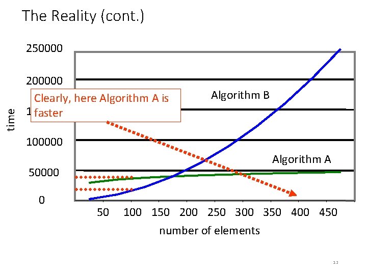
The Reality (cont. ) time 250000 200000 Clearly, here Algorithm A is 150000 faster Algorithm B 100000 Algorithm A 50000 0 50 100 150 200 250 300 350 400 450 number of elements 12

The Reality (cont. ) • The customer was short-changed • By knowing time complexities, we can make an informed decision about how the algorithms compare 13

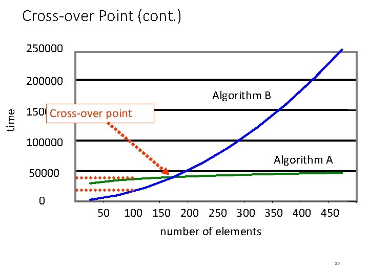
Cross-over Point • The graphs of two algorithms with different time complexities often have a cross-over point… 14

Cross-over Point (cont. ) 250000 time 200000 Algorithm B 150000 Cross-over point 100000 Algorithm A 50000 0 50 100 150 200 250 300 350 400 450 number of elements 15

Cross-over Point (cont. ) • Computer scientists often ignore the left of the cross-over point – the number of elements is low here, so execution time of almost any algorithm is expected to be fast • To the right of the cross-over point, where the number of elements is high, is where people notice the difference in algorithm execution • Asymptotic running time – running time of an algorithm as the number of elements approaches infinity 16

Algorithm Behavior Components • n is used to stand for the number of elements • In reality, it can be anything that has a pronounced effect on execution time of an algorithm as it is varied • n is often referred to as the problem size • The amount of time an algorithm takes to execute is represented by the number of instructions that are executed 17

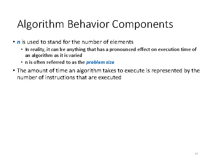
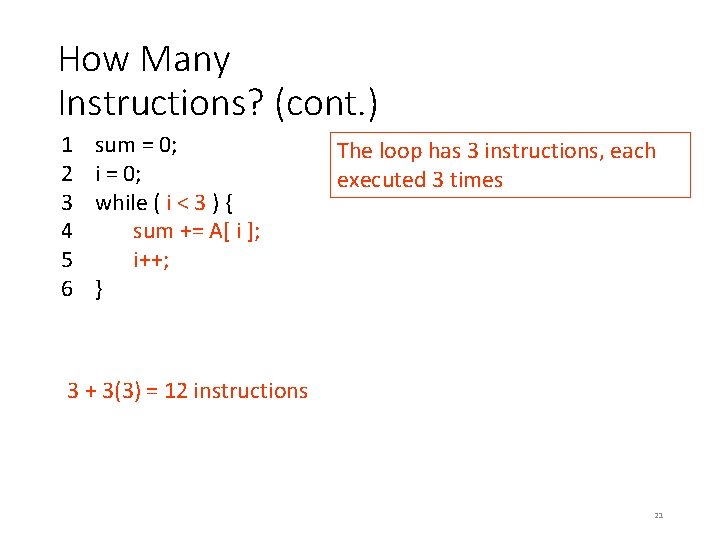
How Many Instructions? 1 2 3 4 5 6 sum = 0; i = 0; while ( i < 3 ) { sum += A[ i ]; i++; } 18

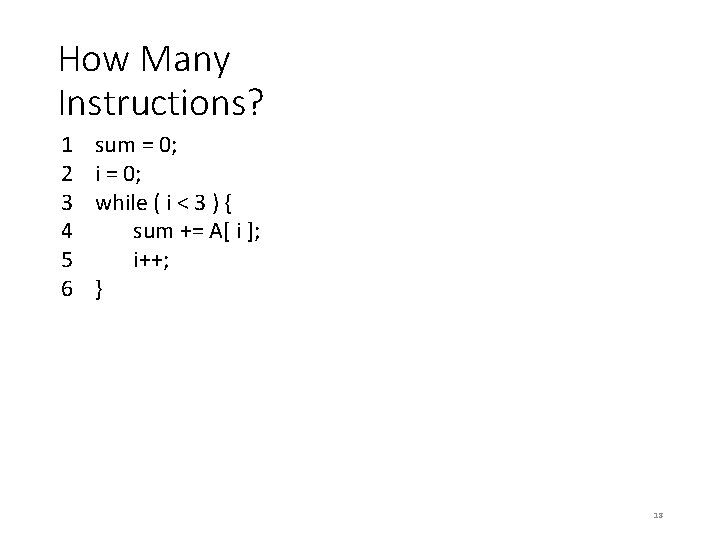
How Many Instructions? (cont. ) 1 2 3 4 5 6 sum = 0; i = 0; while ( i < 3 ) { sum += A[ i ]; i++; } 3 instructions to this point 3+ 19

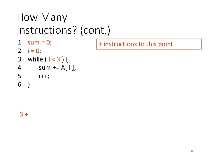
How Many Instructions? (cont. ) 1 2 3 4 5 6 sum = 0; i = 0; while ( i < 3 ) { sum += A[ i ]; i++; } The loop has 3 instructions, each executed 3 times 3+ 20

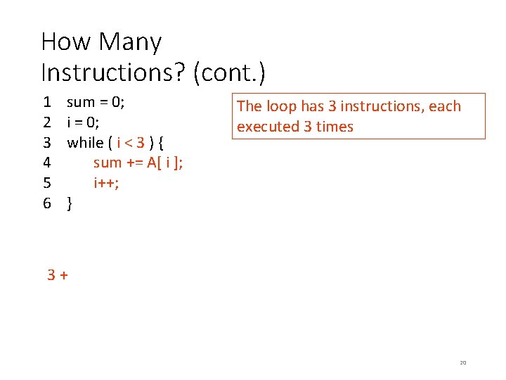
How Many Instructions? (cont. ) 1 2 3 4 5 6 sum = 0; i = 0; while ( i < 3 ) { sum += A[ i ]; i++; } The loop has 3 instructions, each executed 3 times 3 + 3(3) = 12 instructions 21

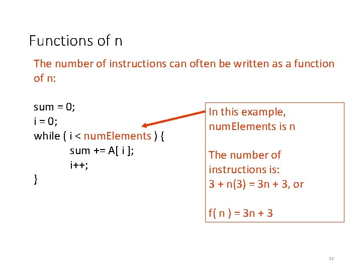
Functions of n The number of instructions can often be written as a function of n: sum = 0; i = 0; while ( i < num. Elements ) { sum += A[ i ]; i++; } In this example, num. Elements is n The number of instructions is: 3 + n(3) = 3 n + 3, or f( n ) = 3 n + 3 22

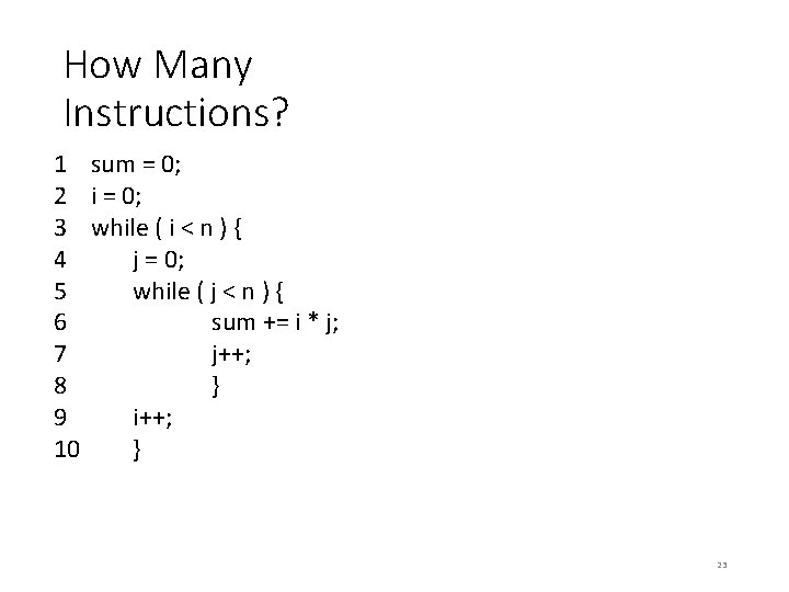
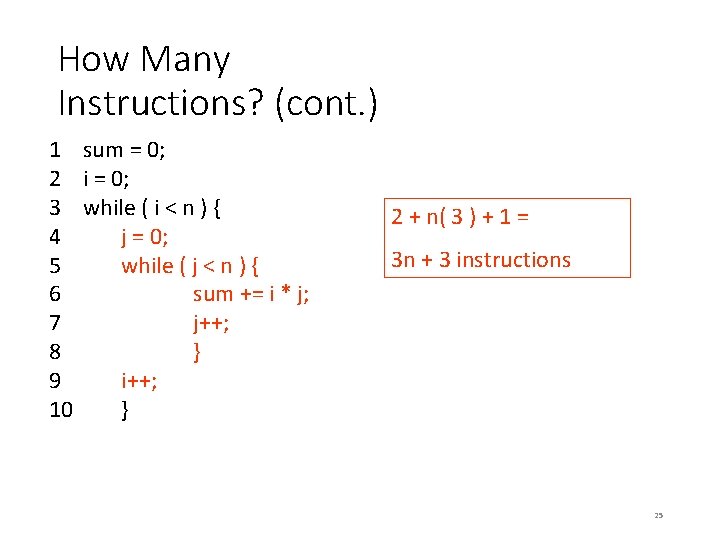
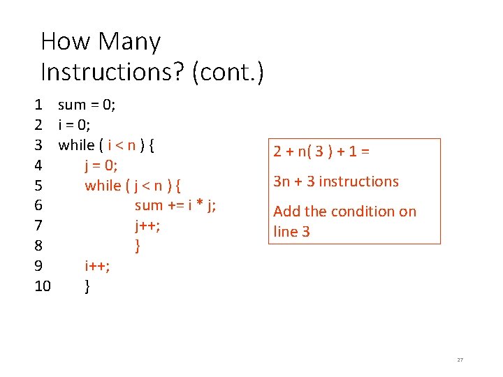
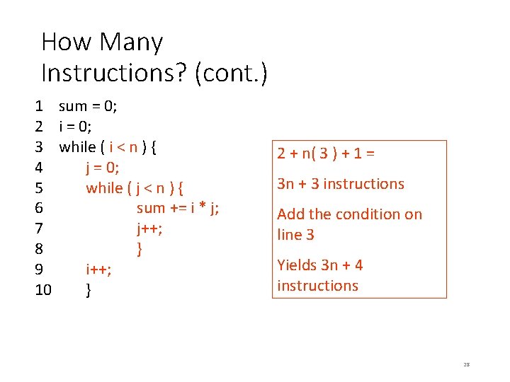
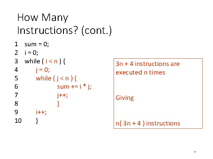
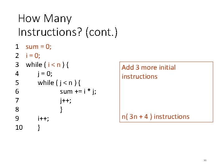
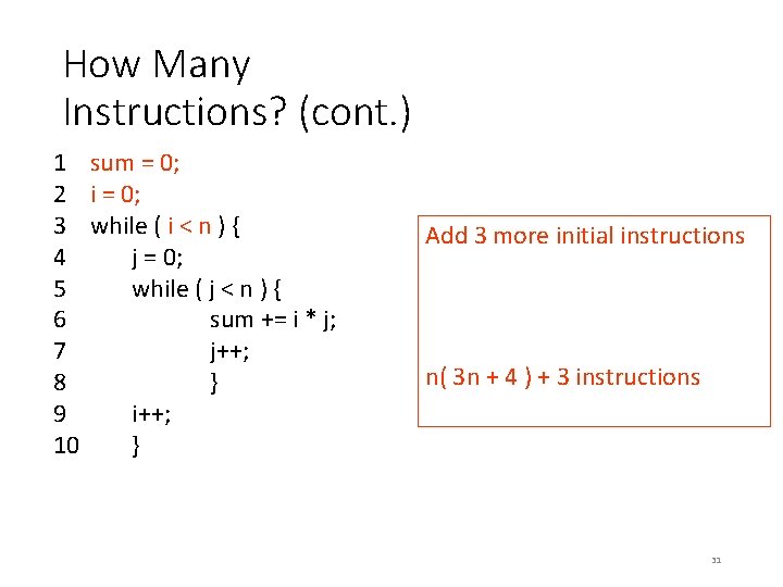
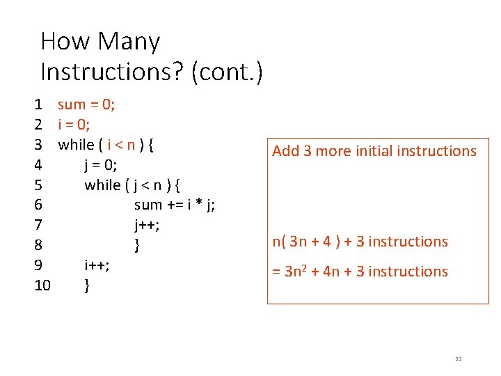
How Many Instructions? 1 sum = 0; 2 i = 0; 3 while ( i < n ) { 4 j = 0; 5 while ( j < n ) { 6 sum += i * j; 7 j++; 8 } 9 i++; 10 } 23

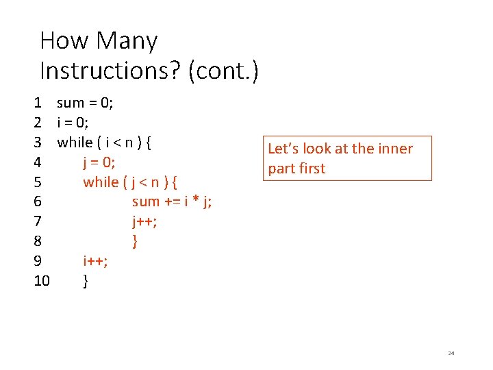
How Many Instructions? (cont. ) 1 sum = 0; 2 i = 0; 3 while ( i < n ) { 4 j = 0; 5 while ( j < n ) { 6 sum += i * j; 7 j++; 8 } 9 i++; 10 } Let’s look at the inner part first 24

How Many Instructions? (cont. ) 1 sum = 0; 2 i = 0; 3 while ( i < n ) { 4 j = 0; 5 while ( j < n ) { 6 sum += i * j; 7 j++; 8 } 9 i++; 10 } 2 + n( 3 ) + 1 = 3 n + 3 instructions 25

How Many Instructions? (cont. ) 1 sum = 0; 2 i = 0; 3 while ( i < n ) { 4 j = 0; 5 while ( j < n ) { 6 sum += i * j; 7 j++; 8 } 9 i++; 10 } 2 + n( 3 ) + 1 = 3 n + 3 instructions Add the condition on line 3 26

How Many Instructions? (cont. ) 1 sum = 0; 2 i = 0; 3 while ( i < n ) { 4 j = 0; 5 while ( j < n ) { 6 sum += i * j; 7 j++; 8 } 9 i++; 10 } 2 + n( 3 ) + 1 = 3 n + 3 instructions Add the condition on line 3 27

How Many Instructions? (cont. ) 1 sum = 0; 2 i = 0; 3 while ( i < n ) { 4 j = 0; 5 while ( j < n ) { 6 sum += i * j; 7 j++; 8 } 9 i++; 10 } 2 + n( 3 ) + 1 = 3 n + 3 instructions Add the condition on line 3 Yields 3 n + 4 instructions 28

How Many Instructions? (cont. ) 1 sum = 0; 2 i = 0; 3 while ( i < n ) { 4 j = 0; 5 while ( j < n ) { 6 sum += i * j; 7 j++; 8 } 9 i++; 10 } 3 n + 4 instructions are executed n times Giving n( 3 n + 4 ) instructions 29

How Many Instructions? (cont. ) 1 sum = 0; 2 i = 0; 3 while ( i < n ) { 4 j = 0; 5 while ( j < n ) { 6 sum += i * j; 7 j++; 8 } 9 i++; 10 } Add 3 more initial instructions n( 3 n + 4 ) instructions 30

How Many Instructions? (cont. ) 1 sum = 0; 2 i = 0; 3 while ( i < n ) { 4 j = 0; 5 while ( j < n ) { 6 sum += i * j; 7 j++; 8 } 9 i++; 10 } Add 3 more initial instructions n( 3 n + 4 ) + 3 instructions 31

How Many Instructions? (cont. ) 1 sum = 0; 2 i = 0; 3 while ( i < n ) { 4 j = 0; 5 while ( j < n ) { 6 sum += i * j; 7 j++; 8 } 9 i++; 10 } Add 3 more initial instructions n( 3 n + 4 ) + 3 instructions = 3 n 2 + 4 n + 3 instructions 32

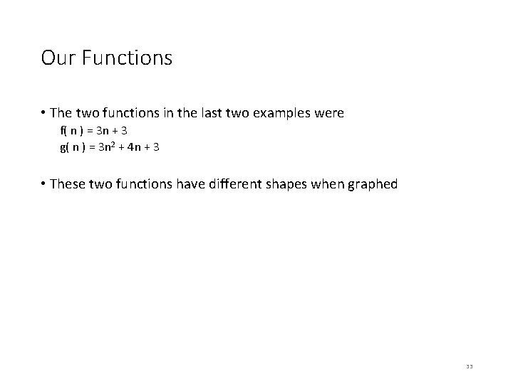
Our Functions • The two functions in the last two examples were f( n ) = 3 n + 3 g( n ) = 3 n 2 + 4 n + 3 • These two functions have different shapes when graphed 33

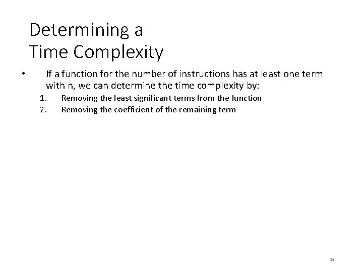
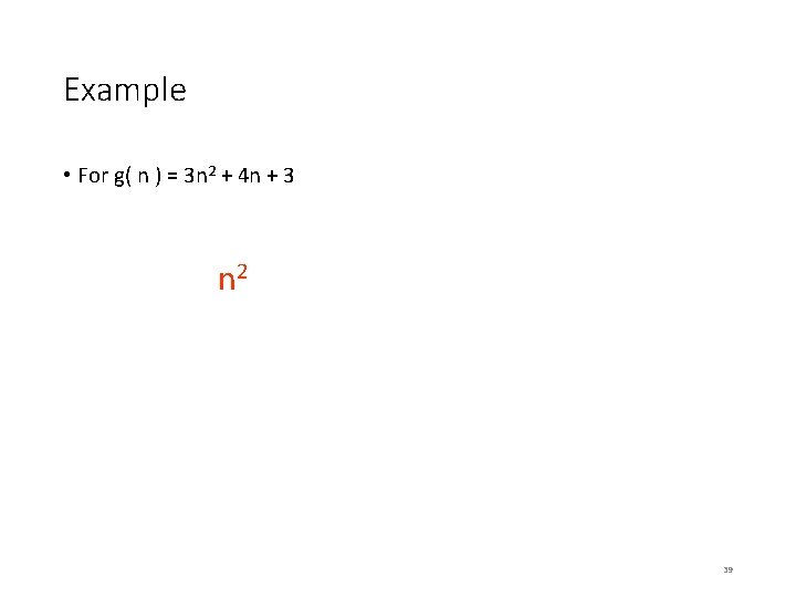
Determining a Time Complexity • If a function for the number of instructions has at least one term with n, we can determine the time complexity by: 1. 2. Removing the least significant terms from the function Removing the coefficient of the remaining term 34

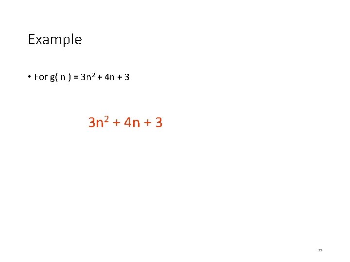
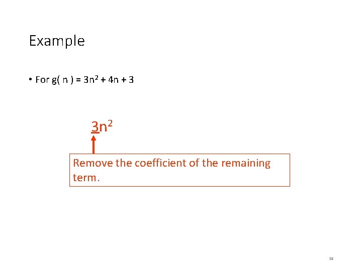
Example • For g( n ) = 3 n 2 + 4 n + 3 35

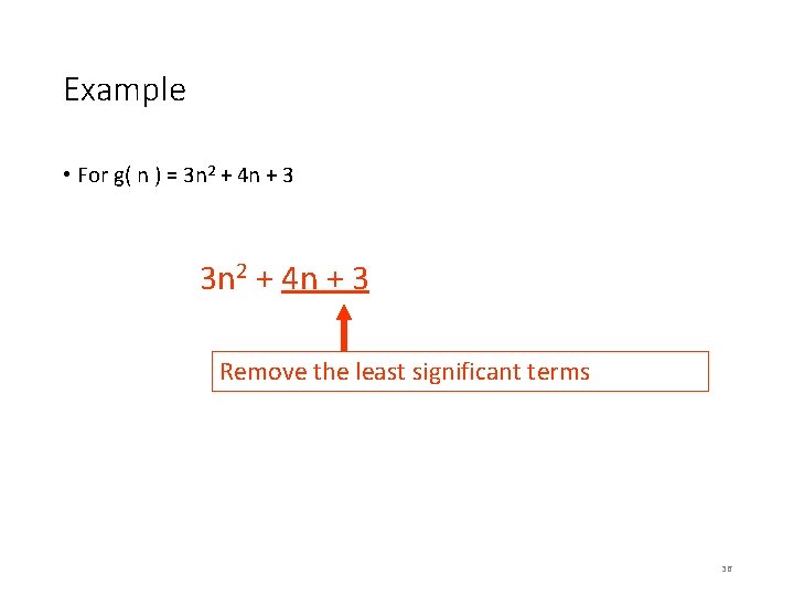
Example • For g( n ) = 3 n 2 + 4 n + 3 Remove the least significant terms 36

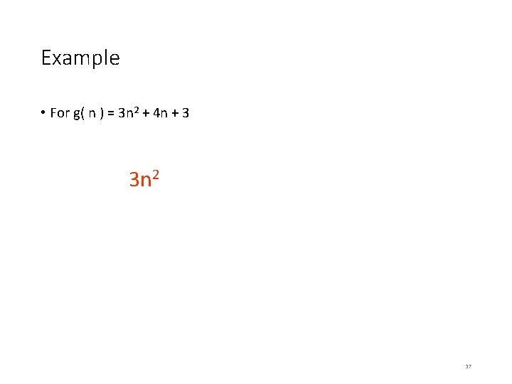
Example • For g( n ) = 3 n 2 + 4 n + 3 3 n 2 37

Example • For g( n ) = 3 n 2 + 4 n + 3 3 n 2 Remove the coefficient of the remaining term. 38

Example • For g( n ) = 3 n 2 + 4 n + 3 3 n 2 39

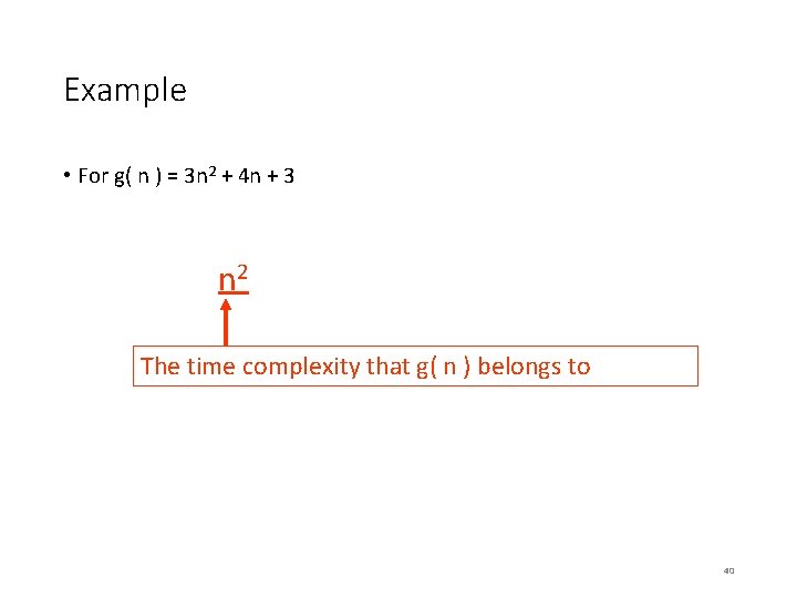
Example • For g( n ) = 3 n 2 + 4 n + 3 3 n 2 The time complexity that g( n ) belongs to 40

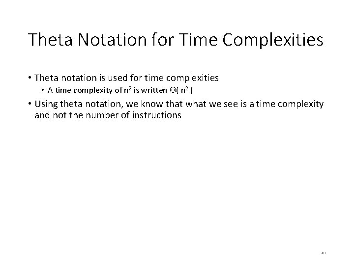
Theta Notation for Time Complexities • Theta notation is used for time complexities • A time complexity of n 2 is written ( n 2 ) • Using theta notation, we know that we see is a time complexity and not the number of instructions 41

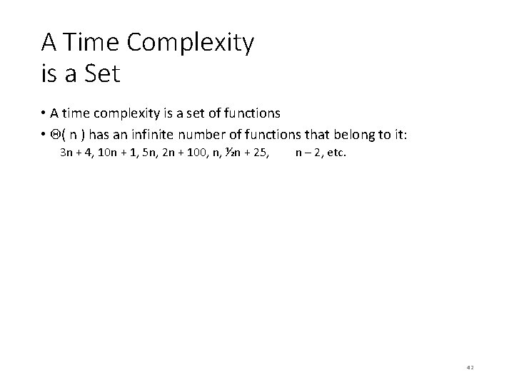
A Time Complexity is a Set • A time complexity is a set of functions • ( n ) has an infinite number of functions that belong to it: 3 n + 4, 10 n + 1, 5 n, 2 n + 100, n, ½n + 25, n – 2, etc. 42

How Different Time Complexities Compare • If two functions belong to two different time complexities, then to the right of the cross-over point: • One will be faster than the other • As n is increased further, more benefit will be gained from the faster function 43

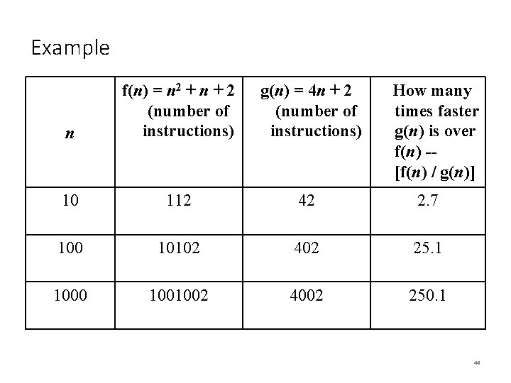
Example n f(n) = n 2 + n + 2 (number of instructions) g(n) = 4 n + 2 (number of instructions) How many times faster g(n) is over f(n) -[f(n) / g(n)] 10 112 42 2. 7 100 10102 402 25. 1 1000 1001002 4002 250. 1 44

Constant Time Complexity • The constant time complexity, written ( 1 ), is the best possible time complexity • As n increases, there is generally no effect on the number of instructions executed • Example: the algorithm which dequeues from the linked list implementation of a queue 45

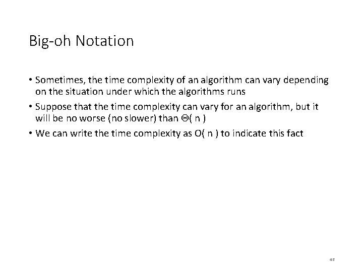
Big-oh Notation • Sometimes, the time complexity of an algorithm can vary depending on the situation under which the algorithms runs • Suppose that the time complexity can vary for an algorithm, but it will be no worse (no slower) than ( n ) • We can write the time complexity as O( n ) to indicate this fact 46

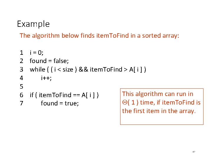
Example The algorithm below finds item. To. Find in a sorted array: 1 2 3 4 5 6 7 i = 0; found = false; while ( ( i < size ) && item. To. Find > A[ i ] ) i++; if ( item. To. Find == A[ i ] ) found = true; This algorithm can run in ( 1 ) time, if item. To. Find is the first item in the array. 47

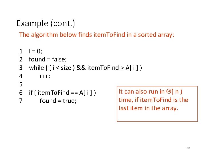
Example (cont. ) The algorithm below finds item. To. Find in a sorted array: 1 2 3 4 5 6 7 i = 0; found = false; while ( ( i < size ) && item. To. Find > A[ i ] ) i++; if ( item. To. Find == A[ i ] ) found = true; It can also run in ( n ) time, if item. To. Find is the last item in the array. 48

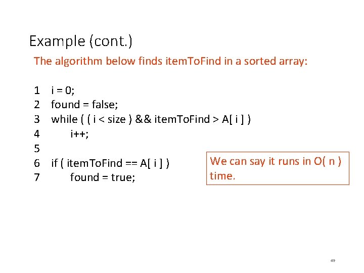
Example (cont. ) The algorithm below finds item. To. Find in a sorted array: 1 2 3 4 5 6 7 i = 0; found = false; while ( ( i < size ) && item. To. Find > A[ i ] ) i++; if ( item. To. Find == A[ i ] ) found = true; We can say it runs in O( n ) time. 49

Logarithmic Equations • A logarithmic equation is just another way of writing an exponential equation… 50

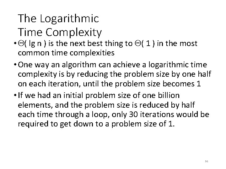
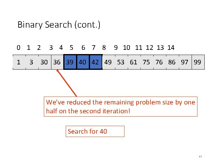
The Logarithmic Time Complexity • ( lg n ) is the next best thing to ( 1 ) in the most common time complexities • One way an algorithm can achieve a logarithmic time complexity is by reducing the problem size by one half on each iteration, until the problem size becomes 1 • If we had an initial problem size of one billion elements, and the problem size is reduced by half each time through a loop, only 30 iterations would be required to get down to a problem size of 1. 51

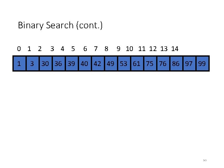
The Binary Search • The binary search algorithm is an example of an algorithm which has a logarithmic time complexity • It searches for an element in a sorted array 52

Binary Search (cont. ) 0 1 2 3 4 5 6 7 8 9 10 11 12 13 14 34 1 34 3 30 36 39 40 42 34 49 34 53 61 75 76 86 97 99 53

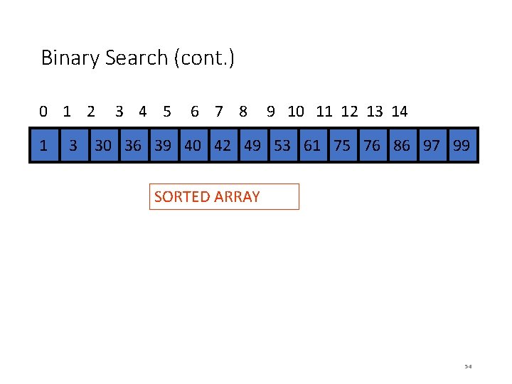
Binary Search (cont. ) 0 1 2 3 4 5 6 7 8 9 10 11 12 13 14 34 1 34 3 30 36 39 40 42 34 49 34 53 61 75 76 86 97 99 SORTED ARRAY 54

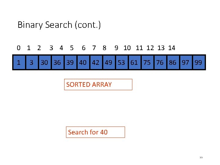
Binary Search (cont. ) 0 1 2 3 4 5 6 7 8 9 10 11 12 13 14 34 1 34 3 30 36 39 40 42 34 49 34 53 61 75 76 86 97 99 SORTED ARRAY Search for 40 55

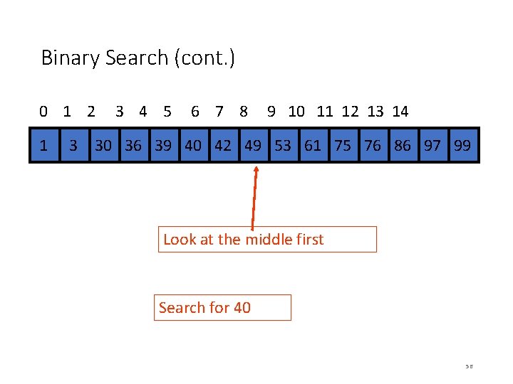
Binary Search (cont. ) 0 1 2 3 4 5 6 7 8 9 10 11 12 13 14 34 1 34 3 30 36 39 40 42 34 49 34 53 61 75 76 86 97 99 Look at the middle first Search for 40 56

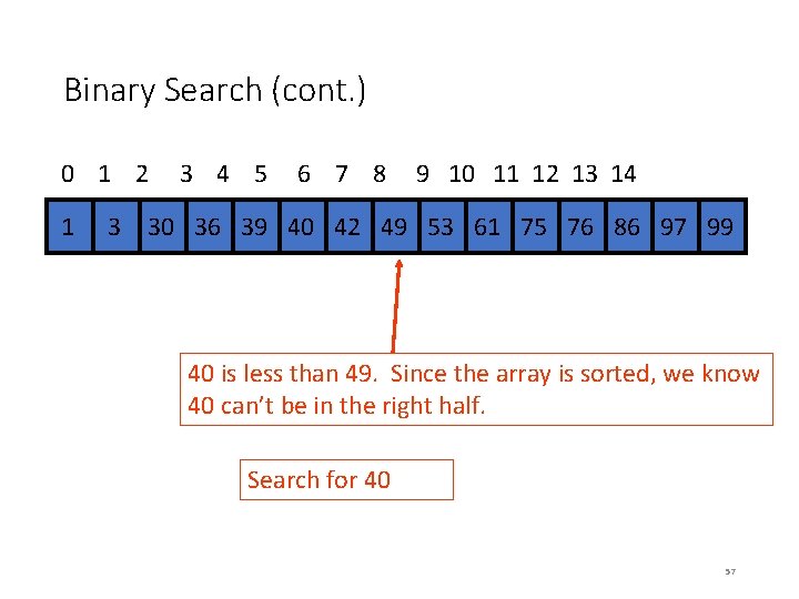
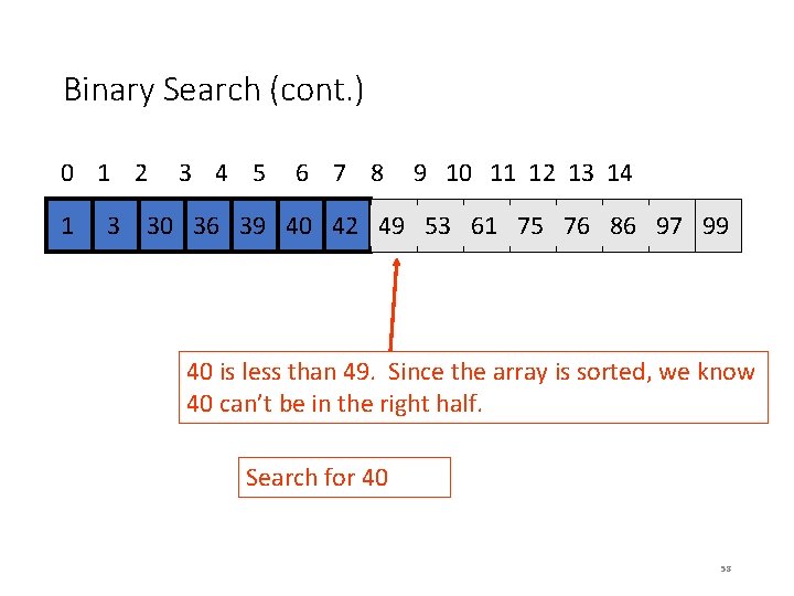
Binary Search (cont. ) 0 1 2 3 4 5 6 7 8 9 10 11 12 13 14 34 1 34 3 30 36 39 40 42 34 49 34 53 61 75 76 86 97 99 40 is less than 49. Since the array is sorted, we know 40 can’t be in the right half. Search for 40 57

Binary Search (cont. ) 0 1 2 3 4 5 6 7 8 9 10 11 12 13 14 34 1 34 3 30 36 39 40 42 34 49 34 53 61 75 76 86 97 99 40 is less than 49. Since the array is sorted, we know 40 can’t be in the right half. Search for 40 58

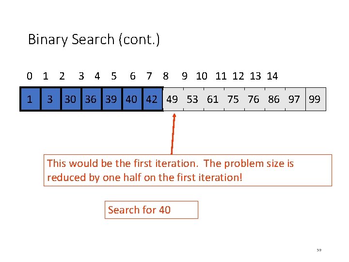
Binary Search (cont. ) 0 1 2 3 4 5 6 7 8 9 10 11 12 13 14 34 1 34 3 30 36 39 40 42 34 49 34 53 61 75 76 86 97 99 This would be the first iteration. The problem size is reduced by one half on the first iteration! Search for 40 59

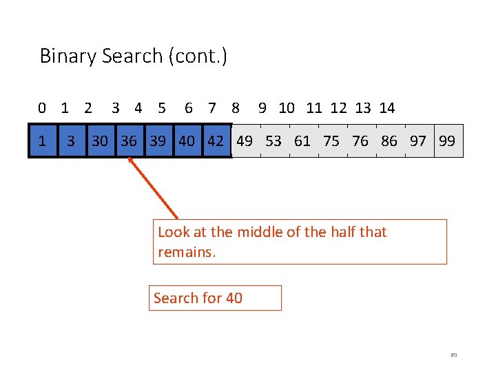
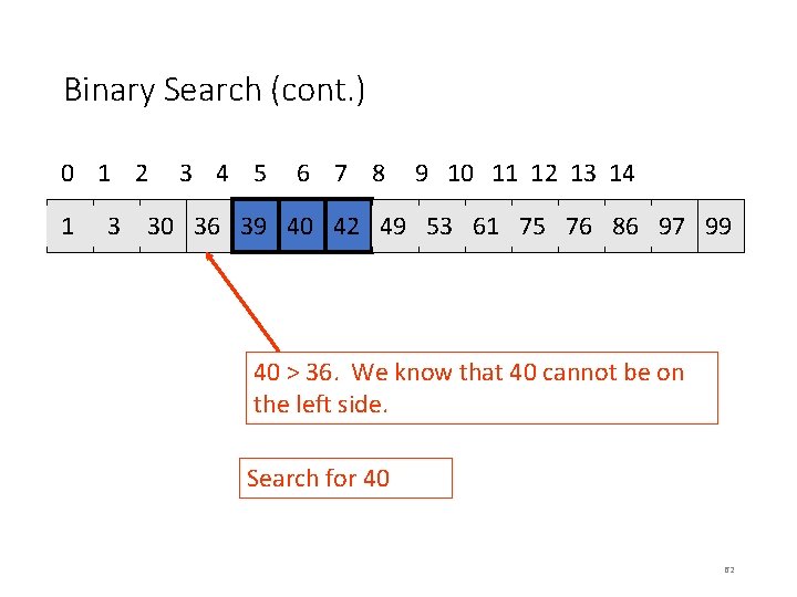
Binary Search (cont. ) 0 1 2 3 4 5 6 7 8 9 10 11 12 13 14 34 1 34 3 30 36 39 40 42 34 49 34 53 61 75 76 86 97 99 Look at the middle of the half that remains. Search for 40 60

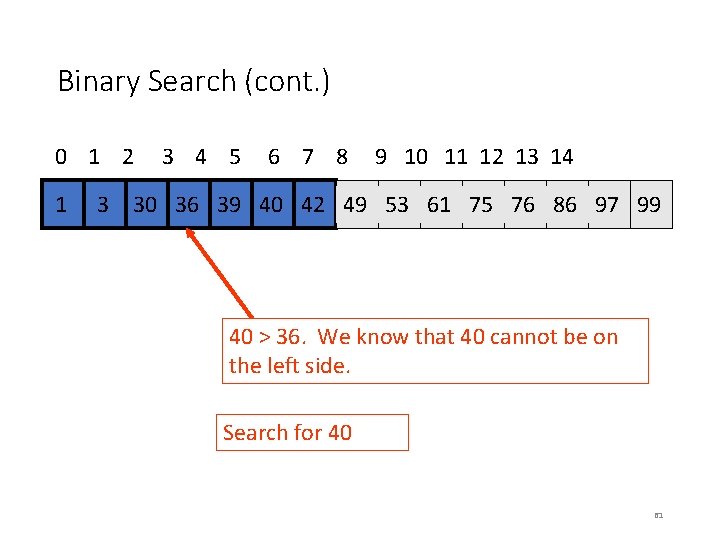
Binary Search (cont. ) 0 1 2 3 4 5 6 7 8 9 10 11 12 13 14 34 1 34 3 30 36 39 40 42 34 49 34 53 61 75 76 86 97 99 40 > 36. We know that 40 cannot be on the left side. Search for 40 61

Binary Search (cont. ) 0 1 2 3 4 5 6 7 8 9 10 11 12 13 14 34 1 34 3 30 36 39 40 42 34 49 34 53 61 75 76 86 97 99 40 > 36. We know that 40 cannot be on the left side. Search for 40 62

Binary Search (cont. ) 0 1 2 3 4 5 6 7 8 9 10 11 12 13 14 34 1 34 3 30 36 39 40 42 34 49 34 53 61 75 76 86 97 99 We’ve reduced the remaining problem size by one half on the second iteration! Search for 40 63

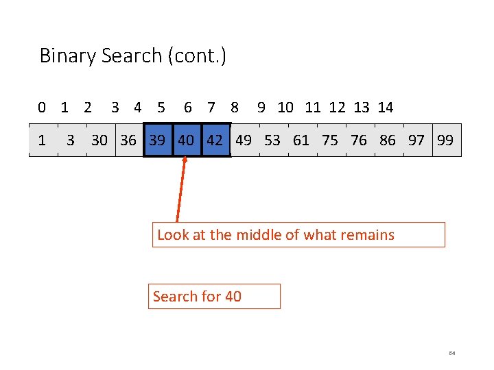
Binary Search (cont. ) 0 1 2 3 4 5 6 7 8 9 10 11 12 13 14 34 1 34 3 30 36 39 40 42 34 49 34 53 61 75 76 86 97 99 Look at the middle of what remains Search for 40 64

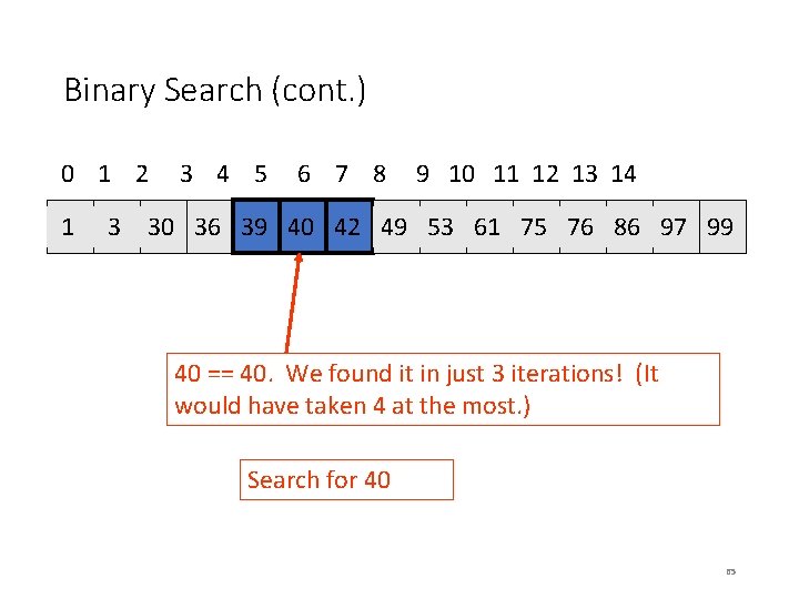
Binary Search (cont. ) 0 1 2 3 4 5 6 7 8 9 10 11 12 13 14 34 1 34 3 30 36 39 40 42 34 49 34 53 61 75 76 86 97 99 40 == 40. We found it in just 3 iterations! (It would have taken 4 at the most. ) Search for 40 65

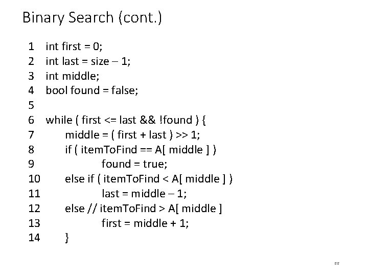
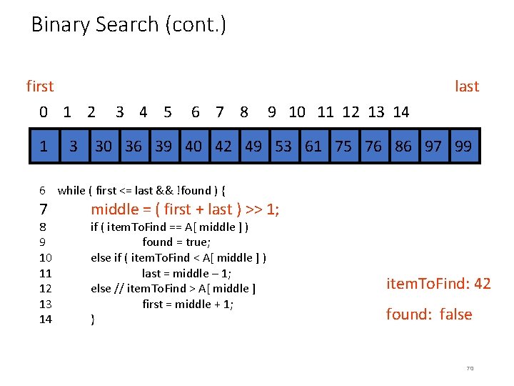
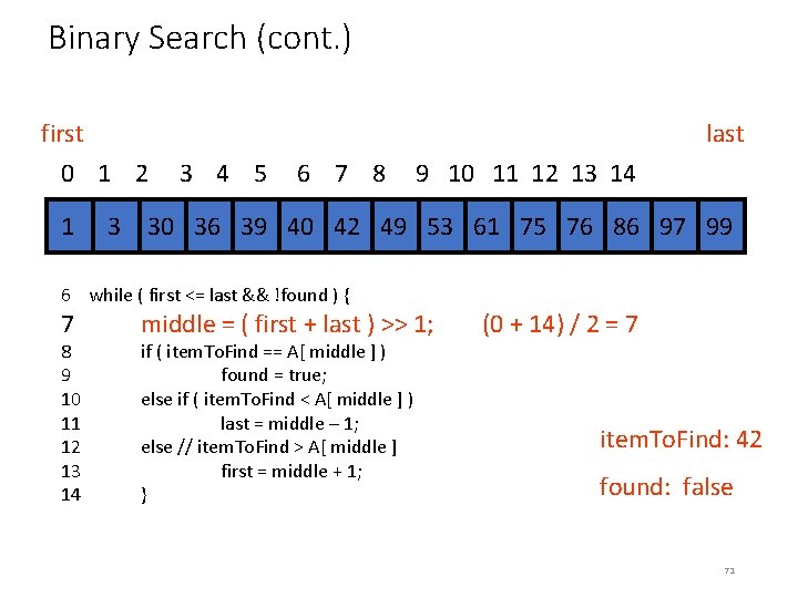
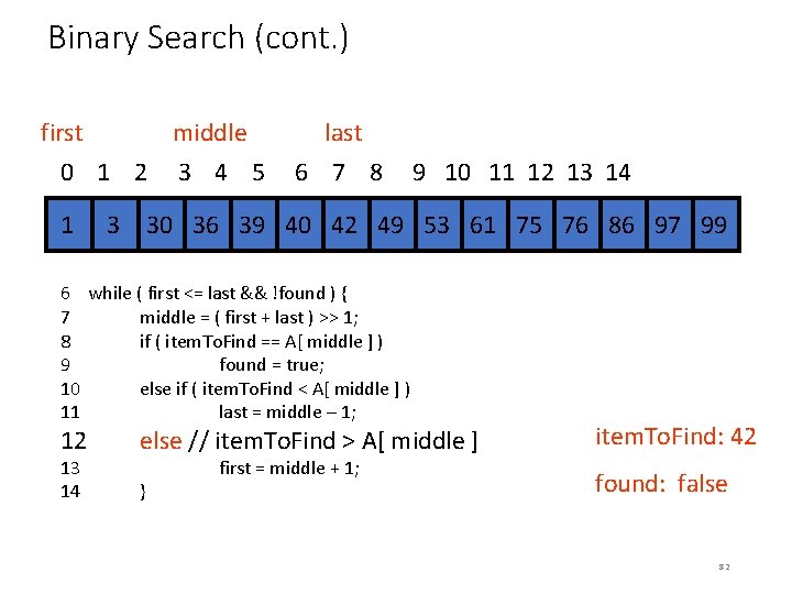
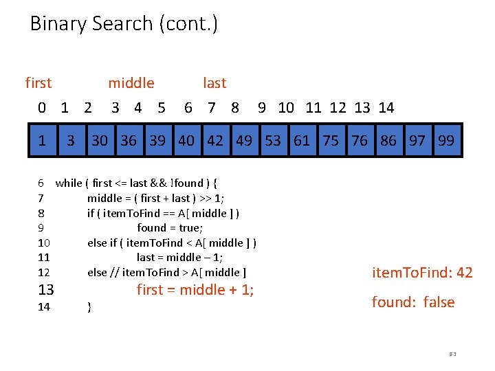
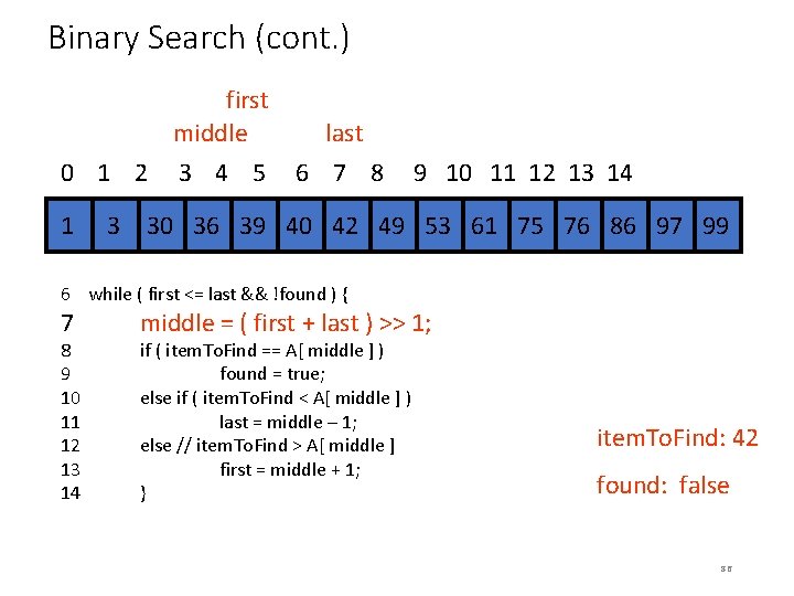
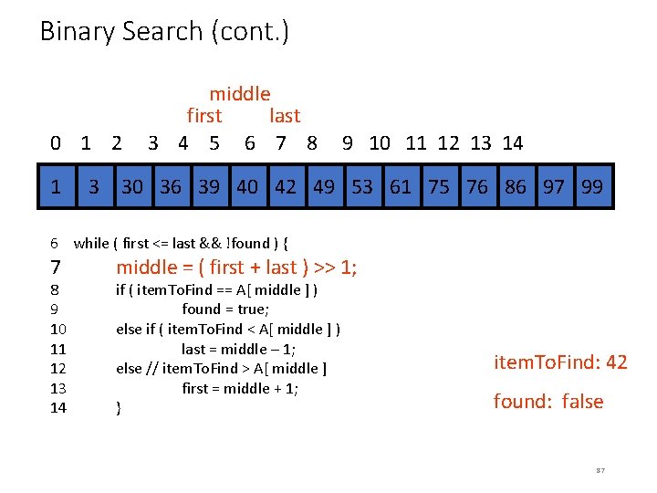
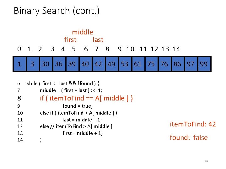
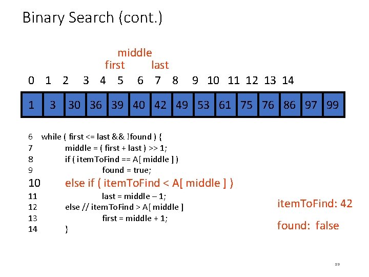
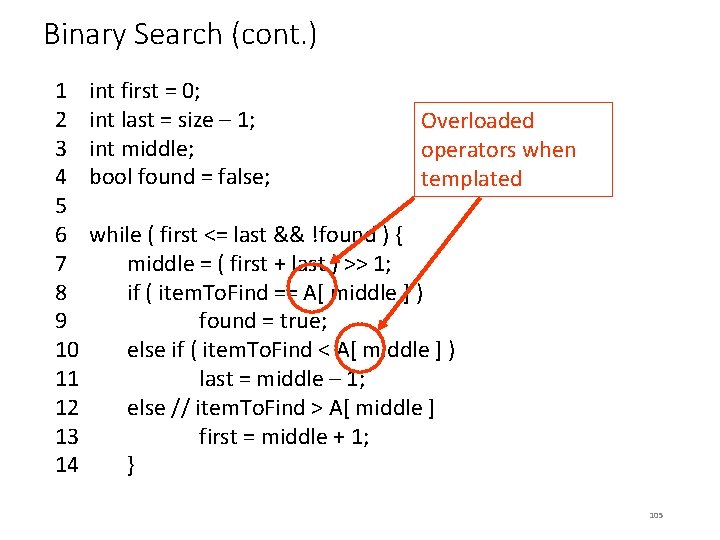
Binary Search (cont. ) 1 2 3 4 5 6 7 8 9 10 11 12 13 14 int first = 0; int last = size – 1; int middle; bool found = false; while ( first <= last && !found ) { middle = ( first + last ) >> 1; if ( item. To. Find == A[ middle ] ) found = true; else if ( item. To. Find < A[ middle ] ) last = middle – 1; else // item. To. Find > A[ middle ] first = middle + 1; } 66

Binary Search (cont. ) 1 2 3 4 5 6 7 8 9 10 11 12 13 14 int first = 0; int last = size – 1; int middle; bool found = false; while ( first <= last && !found ) { middle = ( first + last ) >> 1; if ( item. To. Find == A[ middle ] ) found = true; else if ( item. To. Find < A[ middle ] ) last = middle – 1; else // item. To. Find > A[ middle ] first = middle + 1; } 67

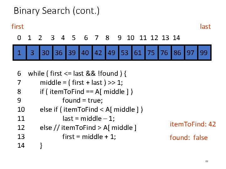
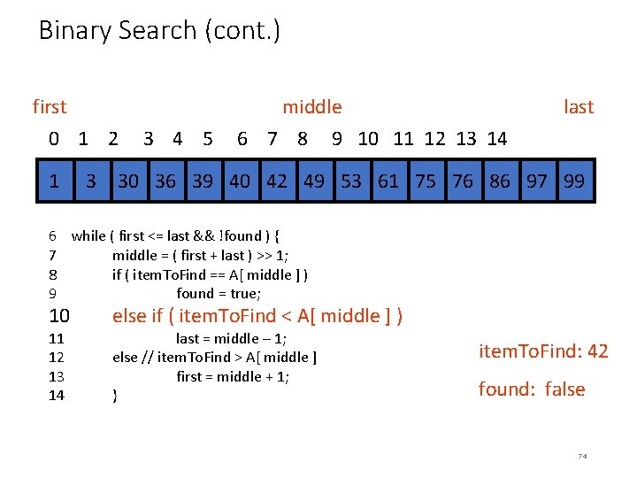
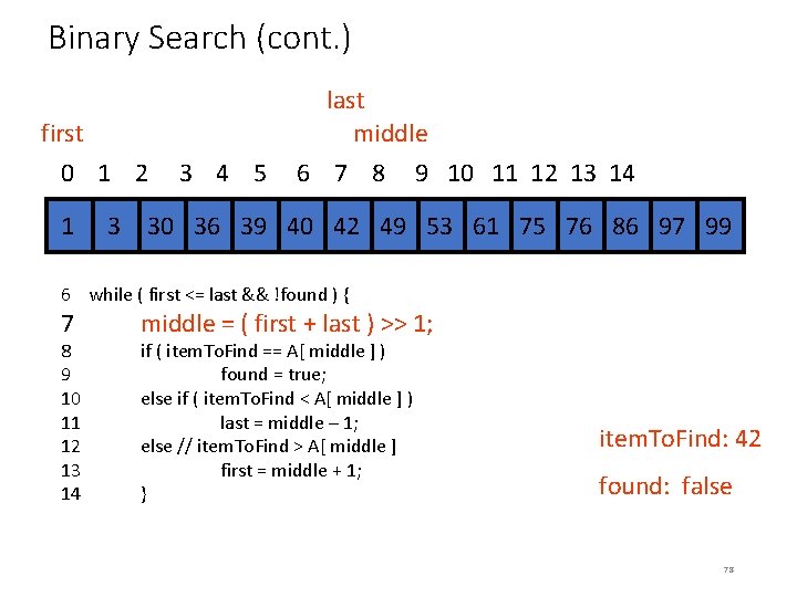
Binary Search (cont. ) first 0 1 2 last 3 4 5 6 7 8 9 10 11 12 13 14 34 1 34 3 30 36 39 40 42 34 49 34 53 61 75 76 86 97 99 6 while ( first <= last && !found ) { 7 middle = ( first + last ) >> 1; 8 if ( item. To. Find == A[ middle ] ) 9 found = true; 10 else if ( item. To. Find < A[ middle ] ) 11 last = middle – 1; 12 else // item. To. Find > A[ middle ] 13 first = middle + 1; 14 } item. To. Find: 42 found: false 68

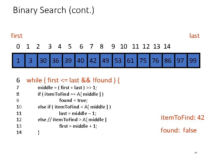
Binary Search (cont. ) first last 0 1 2 3 4 5 6 7 8 9 10 11 12 13 14 34 1 34 3 30 36 39 40 42 34 49 34 53 61 75 76 86 97 99 6 while ( first <= last && !found ) { 7 8 9 10 11 12 13 14 middle = ( first + last ) >> 1; if ( item. To. Find == A[ middle ] ) found = true; else if ( item. To. Find < A[ middle ] ) last = middle – 1; else // item. To. Find > A[ middle ] first = middle + 1; } item. To. Find: 42 found: false 69

Binary Search (cont. ) first last 0 1 2 3 4 5 6 7 8 9 10 11 12 13 14 34 1 34 3 30 36 39 40 42 34 49 34 53 61 75 76 86 97 99 6 while ( first <= last && !found ) { 7 8 9 10 11 12 13 14 middle = ( first + last ) >> 1; if ( item. To. Find == A[ middle ] ) found = true; else if ( item. To. Find < A[ middle ] ) last = middle – 1; else // item. To. Find > A[ middle ] first = middle + 1; } item. To. Find: 42 found: false 70

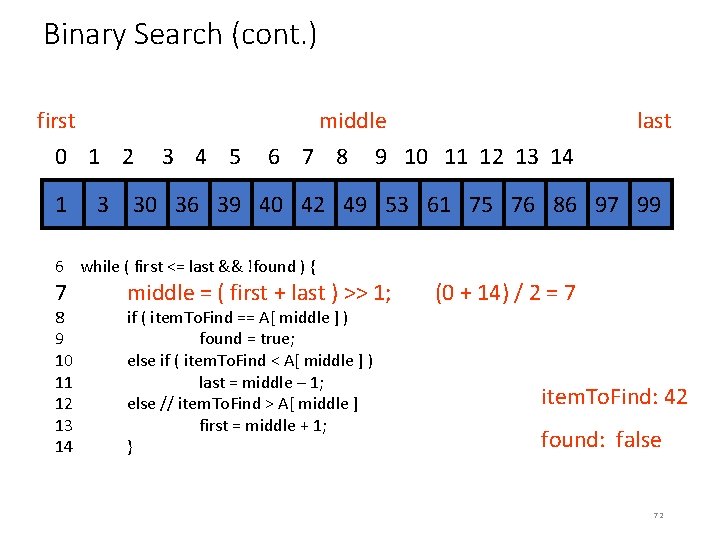
Binary Search (cont. ) first last 0 1 2 3 4 5 6 7 8 9 10 11 12 13 14 34 1 34 3 30 36 39 40 42 34 49 34 53 61 75 76 86 97 99 6 while ( first <= last && !found ) { 7 8 9 10 11 12 13 14 middle = ( first + last ) >> 1; if ( item. To. Find == A[ middle ] ) found = true; else if ( item. To. Find < A[ middle ] ) last = middle – 1; else // item. To. Find > A[ middle ] first = middle + 1; } (0 + 14) / 2 = 7 item. To. Find: 42 found: false 71

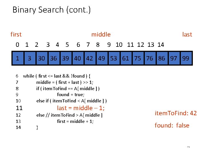
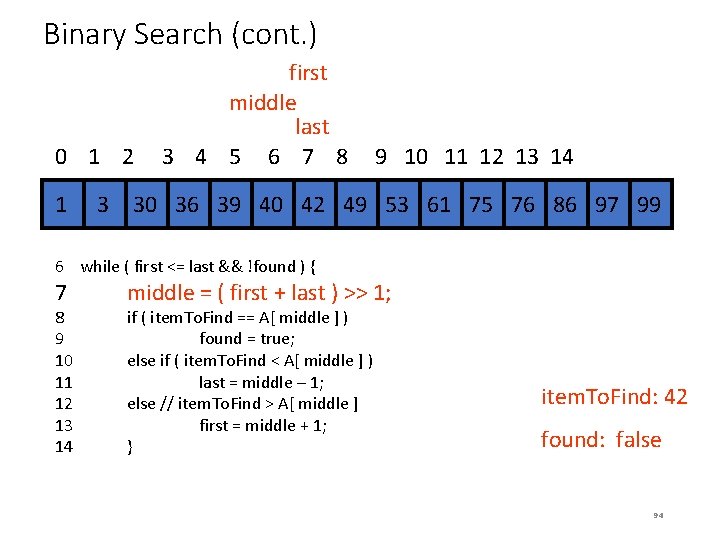
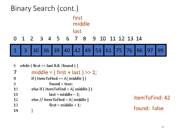
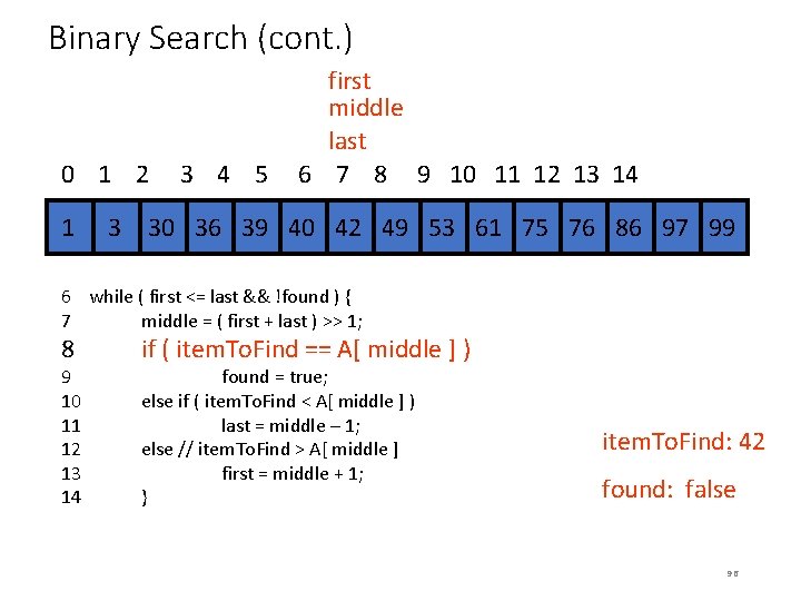
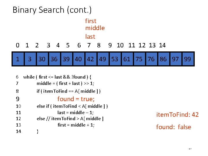
Binary Search (cont. ) first middle 0 1 2 3 4 5 6 7 8 last 9 10 11 12 13 14 34 1 34 3 30 36 39 40 42 34 49 34 53 61 75 76 86 97 99 6 while ( first <= last && !found ) { 7 8 9 10 11 12 13 14 middle = ( first + last ) >> 1; if ( item. To. Find == A[ middle ] ) found = true; else if ( item. To. Find < A[ middle ] ) last = middle – 1; else // item. To. Find > A[ middle ] first = middle + 1; } (0 + 14) / 2 = 7 item. To. Find: 42 found: false 72

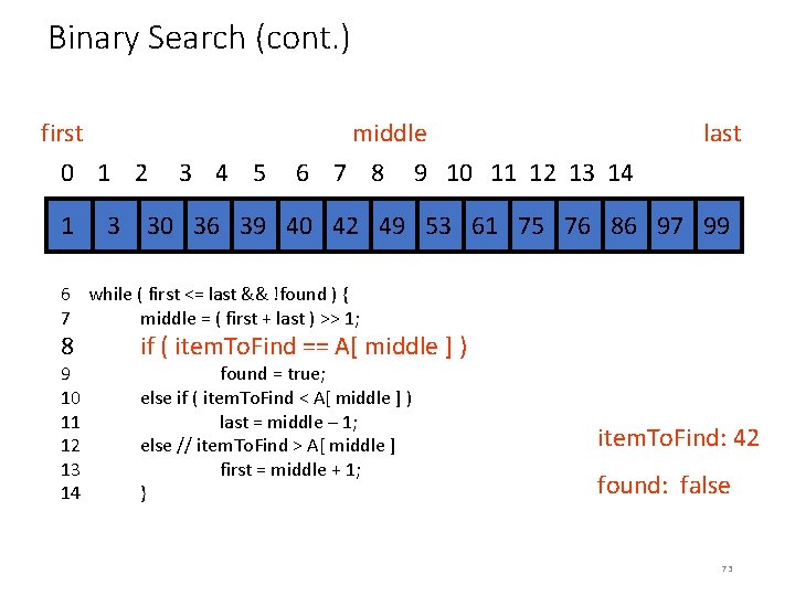
Binary Search (cont. ) first middle 0 1 2 3 4 5 6 7 8 last 9 10 11 12 13 14 34 1 34 3 30 36 39 40 42 34 49 34 53 61 75 76 86 97 99 6 while ( first <= last && !found ) { 7 middle = ( first + last ) >> 1; 8 9 10 11 12 13 14 if ( item. To. Find == A[ middle ] ) found = true; else if ( item. To. Find < A[ middle ] ) last = middle – 1; else // item. To. Find > A[ middle ] first = middle + 1; } item. To. Find: 42 found: false 73

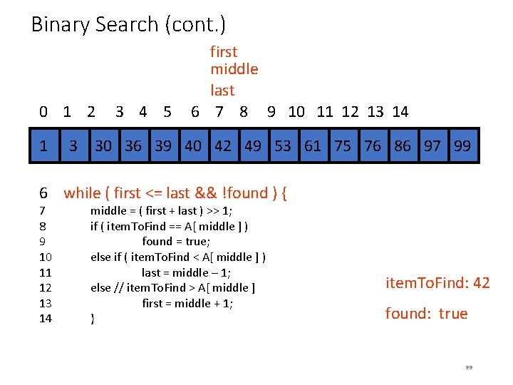
Binary Search (cont. ) first middle 0 1 2 3 4 5 6 7 8 last 9 10 11 12 13 14 34 1 34 3 30 36 39 40 42 34 49 34 53 61 75 76 86 97 99 6 while ( first <= last && !found ) { 7 middle = ( first + last ) >> 1; 8 if ( item. To. Find == A[ middle ] ) 9 found = true; 10 11 12 13 14 else if ( item. To. Find < A[ middle ] ) last = middle – 1; else // item. To. Find > A[ middle ] first = middle + 1; } item. To. Find: 42 found: false 74

Binary Search (cont. ) first middle 0 1 2 3 4 5 6 7 8 last 9 10 11 12 13 14 34 1 34 3 30 36 39 40 42 34 49 34 53 61 75 76 86 97 99 6 while ( first <= last && !found ) { 7 middle = ( first + last ) >> 1; 8 if ( item. To. Find == A[ middle ] ) 9 found = true; 10 else if ( item. To. Find < A[ middle ] ) 11 12 13 14 last = middle – 1; else // item. To. Find > A[ middle ] first = middle + 1; } item. To. Find: 42 found: false 75

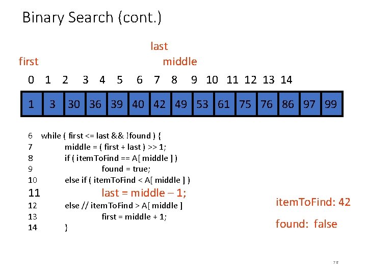
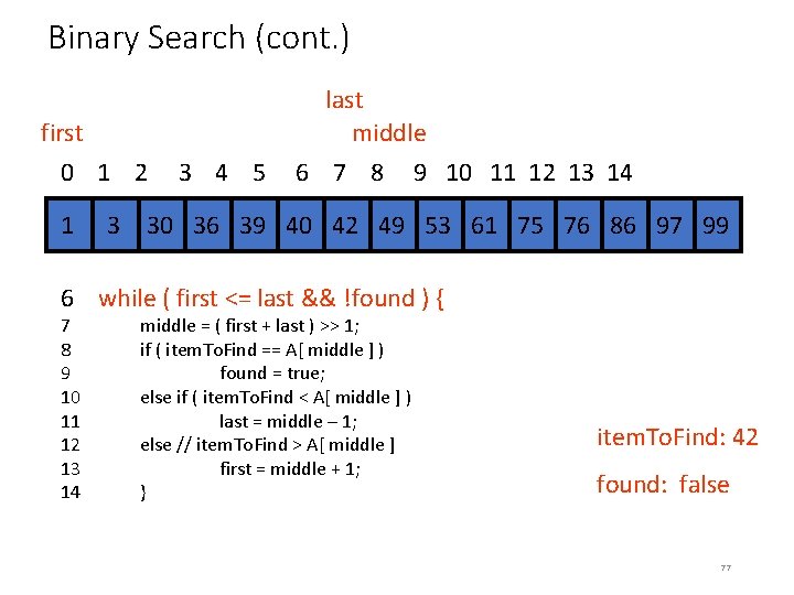
Binary Search (cont. ) last middle first 0 1 2 3 4 5 6 7 8 9 10 11 12 13 14 34 1 34 3 30 36 39 40 42 34 49 34 53 61 75 76 86 97 99 6 while ( first <= last && !found ) { 7 middle = ( first + last ) >> 1; 8 if ( item. To. Find == A[ middle ] ) 9 found = true; 10 else if ( item. To. Find < A[ middle ] ) 11 12 13 14 last = middle – 1; else // item. To. Find > A[ middle ] first = middle + 1; } item. To. Find: 42 found: false 76

Binary Search (cont. ) last middle first 0 1 2 3 4 5 6 7 8 9 10 11 12 13 14 34 1 34 3 30 36 39 40 42 34 49 34 53 61 75 76 86 97 99 6 while ( first <= last && !found ) { 7 8 9 10 11 12 13 14 middle = ( first + last ) >> 1; if ( item. To. Find == A[ middle ] ) found = true; else if ( item. To. Find < A[ middle ] ) last = middle – 1; else // item. To. Find > A[ middle ] first = middle + 1; } item. To. Find: 42 found: false 77

Binary Search (cont. ) last middle first 0 1 2 3 4 5 6 7 8 9 10 11 12 13 14 34 1 34 3 30 36 39 40 42 34 49 34 53 61 75 76 86 97 99 6 while ( first <= last && !found ) { 7 8 9 10 11 12 13 14 middle = ( first + last ) >> 1; if ( item. To. Find == A[ middle ] ) found = true; else if ( item. To. Find < A[ middle ] ) last = middle – 1; else // item. To. Find > A[ middle ] first = middle + 1; } item. To. Find: 42 found: false 78

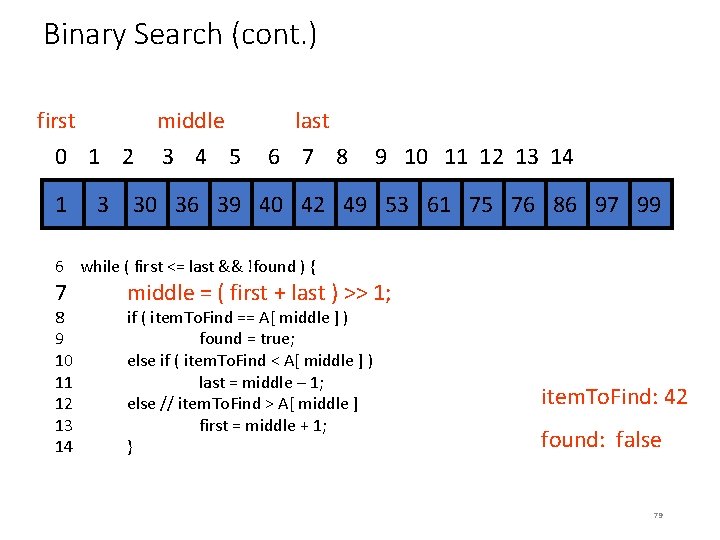
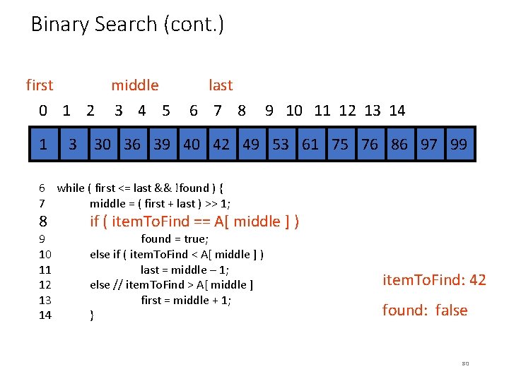
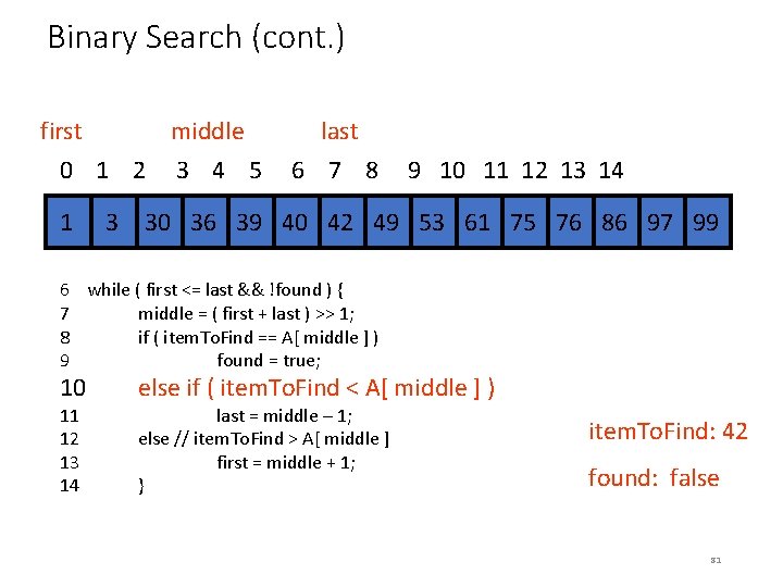
Binary Search (cont. ) first middle 0 1 2 3 4 5 last 6 7 8 9 10 11 12 13 14 34 1 34 3 30 36 39 40 42 34 49 34 53 61 75 76 86 97 99 6 while ( first <= last && !found ) { 7 8 9 10 11 12 13 14 middle = ( first + last ) >> 1; if ( item. To. Find == A[ middle ] ) found = true; else if ( item. To. Find < A[ middle ] ) last = middle – 1; else // item. To. Find > A[ middle ] first = middle + 1; } item. To. Find: 42 found: false 79

Binary Search (cont. ) first middle 0 1 2 3 4 5 last 6 7 8 9 10 11 12 13 14 34 1 34 3 30 36 39 40 42 34 49 34 53 61 75 76 86 97 99 6 while ( first <= last && !found ) { 7 middle = ( first + last ) >> 1; 8 9 10 11 12 13 14 if ( item. To. Find == A[ middle ] ) found = true; else if ( item. To. Find < A[ middle ] ) last = middle – 1; else // item. To. Find > A[ middle ] first = middle + 1; } item. To. Find: 42 found: false 80

Binary Search (cont. ) first middle 0 1 2 3 4 5 last 6 7 8 9 10 11 12 13 14 34 1 34 3 30 36 39 40 42 34 49 34 53 61 75 76 86 97 99 6 while ( first <= last && !found ) { 7 middle = ( first + last ) >> 1; 8 if ( item. To. Find == A[ middle ] ) 9 found = true; 10 11 12 13 14 else if ( item. To. Find < A[ middle ] ) last = middle – 1; else // item. To. Find > A[ middle ] first = middle + 1; } item. To. Find: 42 found: false 81

Binary Search (cont. ) first middle 0 1 2 3 4 5 last 6 7 8 9 10 11 12 13 14 34 1 34 3 30 36 39 40 42 34 49 34 53 61 75 76 86 97 99 6 while ( first <= last && !found ) { 7 middle = ( first + last ) >> 1; 8 if ( item. To. Find == A[ middle ] ) 9 found = true; 10 else if ( item. To. Find < A[ middle ] ) 11 last = middle – 1; 12 13 14 else // item. To. Find > A[ middle ] item. To. Find: 42 } found: false first = middle + 1; 82

Binary Search (cont. ) first middle 0 1 2 3 4 5 last 6 7 8 9 10 11 12 13 14 34 1 34 3 30 36 39 40 42 34 49 34 53 61 75 76 86 97 99 6 while ( first <= last && !found ) { 7 middle = ( first + last ) >> 1; 8 if ( item. To. Find == A[ middle ] ) 9 found = true; 10 else if ( item. To. Find < A[ middle ] ) 11 last = middle – 1; 12 else // item. To. Find > A[ middle ] item. To. Find: 42 14 found: false 13 } first = middle + 1; 83

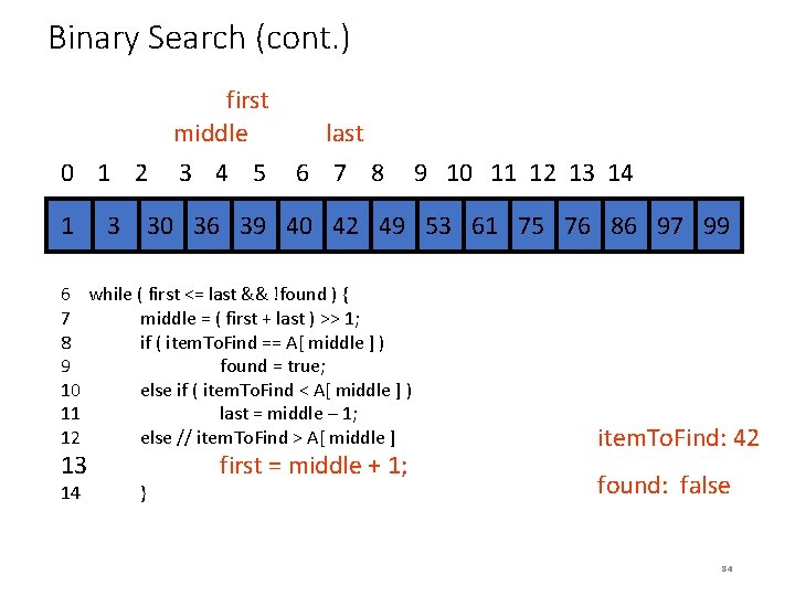
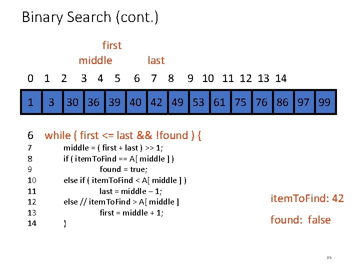
Binary Search (cont. ) 0 1 2 first middle last 3 4 5 6 7 8 9 10 11 12 13 14 34 1 34 3 30 36 39 40 42 34 49 34 53 61 75 76 86 97 99 6 while ( first <= last && !found ) { 7 middle = ( first + last ) >> 1; 8 if ( item. To. Find == A[ middle ] ) 9 found = true; 10 else if ( item. To. Find < A[ middle ] ) 11 last = middle – 1; 12 else // item. To. Find > A[ middle ] item. To. Find: 42 14 found: false 13 } first = middle + 1; 84

Binary Search (cont. ) 0 1 2 first middle last 3 4 5 6 7 8 9 10 11 12 13 14 34 1 34 3 30 36 39 40 42 34 49 34 53 61 75 76 86 97 99 6 while ( first <= last && !found ) { 7 8 9 10 11 12 13 14 middle = ( first + last ) >> 1; if ( item. To. Find == A[ middle ] ) found = true; else if ( item. To. Find < A[ middle ] ) last = middle – 1; else // item. To. Find > A[ middle ] first = middle + 1; } item. To. Find: 42 found: false 85

Binary Search (cont. ) 0 1 2 first middle last 3 4 5 6 7 8 9 10 11 12 13 14 34 1 34 3 30 36 39 40 42 34 49 34 53 61 75 76 86 97 99 6 while ( first <= last && !found ) { 7 8 9 10 11 12 13 14 middle = ( first + last ) >> 1; if ( item. To. Find == A[ middle ] ) found = true; else if ( item. To. Find < A[ middle ] ) last = middle – 1; else // item. To. Find > A[ middle ] first = middle + 1; } item. To. Find: 42 found: false 86

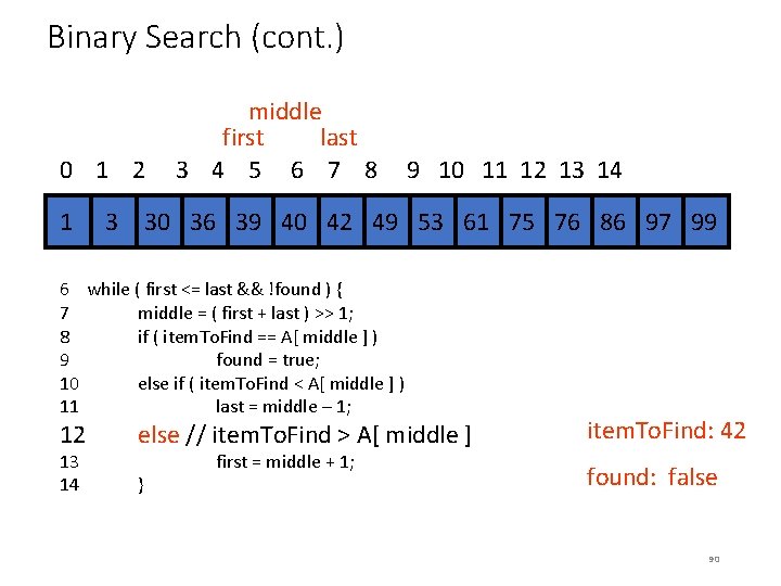
Binary Search (cont. ) 0 1 2 middle first last 3 4 5 6 7 8 9 10 11 12 13 14 34 1 34 3 30 36 39 40 42 34 49 34 53 61 75 76 86 97 99 6 while ( first <= last && !found ) { 7 8 9 10 11 12 13 14 middle = ( first + last ) >> 1; if ( item. To. Find == A[ middle ] ) found = true; else if ( item. To. Find < A[ middle ] ) last = middle – 1; else // item. To. Find > A[ middle ] first = middle + 1; } item. To. Find: 42 found: false 87

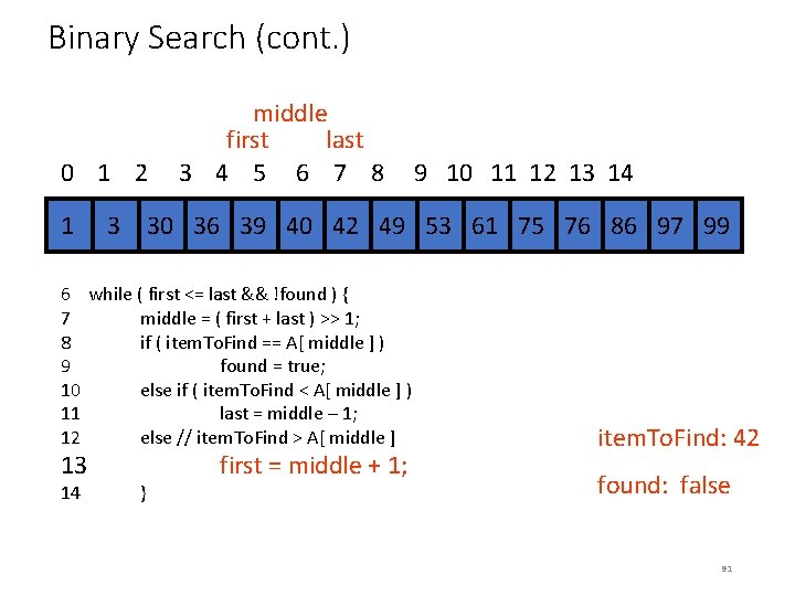
Binary Search (cont. ) 0 1 2 middle first last 3 4 5 6 7 8 9 10 11 12 13 14 34 1 34 3 30 36 39 40 42 34 49 34 53 61 75 76 86 97 99 6 while ( first <= last && !found ) { 7 middle = ( first + last ) >> 1; 8 9 10 11 12 13 14 if ( item. To. Find == A[ middle ] ) found = true; else if ( item. To. Find < A[ middle ] ) last = middle – 1; else // item. To. Find > A[ middle ] first = middle + 1; } item. To. Find: 42 found: false 88

Binary Search (cont. ) 0 1 2 middle first last 3 4 5 6 7 8 9 10 11 12 13 14 34 1 34 3 30 36 39 40 42 34 49 34 53 61 75 76 86 97 99 6 while ( first <= last && !found ) { 7 middle = ( first + last ) >> 1; 8 if ( item. To. Find == A[ middle ] ) 9 found = true; 10 11 12 13 14 else if ( item. To. Find < A[ middle ] ) last = middle – 1; else // item. To. Find > A[ middle ] first = middle + 1; } item. To. Find: 42 found: false 89

Binary Search (cont. ) 0 1 2 middle first last 3 4 5 6 7 8 9 10 11 12 13 14 34 1 34 3 30 36 39 40 42 34 49 34 53 61 75 76 86 97 99 6 while ( first <= last && !found ) { 7 middle = ( first + last ) >> 1; 8 if ( item. To. Find == A[ middle ] ) 9 found = true; 10 else if ( item. To. Find < A[ middle ] ) 11 last = middle – 1; 12 13 14 else // item. To. Find > A[ middle ] item. To. Find: 42 } found: false first = middle + 1; 90

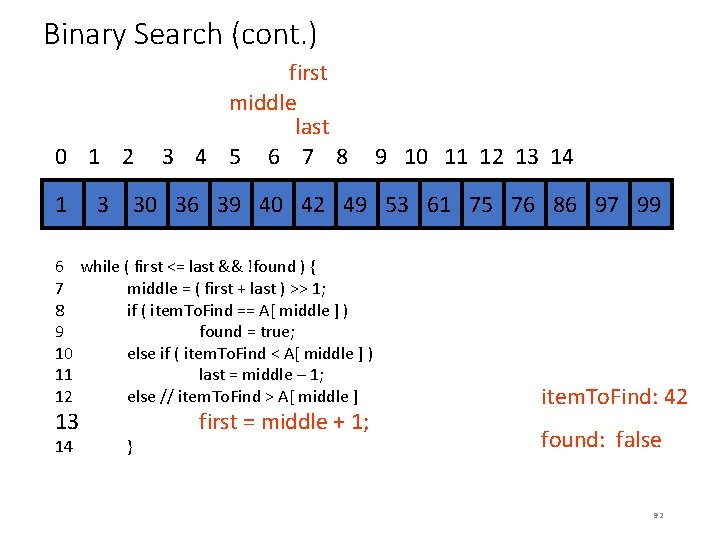
Binary Search (cont. ) 0 1 2 middle first last 3 4 5 6 7 8 9 10 11 12 13 14 34 1 34 3 30 36 39 40 42 34 49 34 53 61 75 76 86 97 99 6 while ( first <= last && !found ) { 7 middle = ( first + last ) >> 1; 8 if ( item. To. Find == A[ middle ] ) 9 found = true; 10 else if ( item. To. Find < A[ middle ] ) 11 last = middle – 1; 12 else // item. To. Find > A[ middle ] item. To. Find: 42 14 found: false 13 } first = middle + 1; 91

Binary Search (cont. ) 0 1 2 first middle last 3 4 5 6 7 8 9 10 11 12 13 14 34 1 34 3 30 36 39 40 42 34 49 34 53 61 75 76 86 97 99 6 while ( first <= last && !found ) { 7 middle = ( first + last ) >> 1; 8 if ( item. To. Find == A[ middle ] ) 9 found = true; 10 else if ( item. To. Find < A[ middle ] ) 11 last = middle – 1; 12 else // item. To. Find > A[ middle ] item. To. Find: 42 14 found: false 13 } first = middle + 1; 92

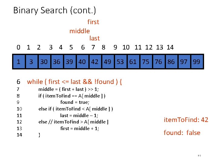
Binary Search (cont. ) 0 1 2 first middle last 3 4 5 6 7 8 9 10 11 12 13 14 34 1 34 3 30 36 39 40 42 34 49 34 53 61 75 76 86 97 99 6 while ( first <= last && !found ) { 7 8 9 10 11 12 13 14 middle = ( first + last ) >> 1; if ( item. To. Find == A[ middle ] ) found = true; else if ( item. To. Find < A[ middle ] ) last = middle – 1; else // item. To. Find > A[ middle ] first = middle + 1; } item. To. Find: 42 found: false 93

Binary Search (cont. ) 0 1 2 first middle last 3 4 5 6 7 8 9 10 11 12 13 14 34 1 34 3 30 36 39 40 42 34 49 34 53 61 75 76 86 97 99 6 while ( first <= last && !found ) { 7 8 9 10 11 12 13 14 middle = ( first + last ) >> 1; if ( item. To. Find == A[ middle ] ) found = true; else if ( item. To. Find < A[ middle ] ) last = middle – 1; else // item. To. Find > A[ middle ] first = middle + 1; } item. To. Find: 42 found: false 94

Binary Search (cont. ) 0 1 2 3 4 5 first middle last 6 7 8 9 10 11 12 13 14 34 1 34 3 30 36 39 40 42 34 49 34 53 61 75 76 86 97 99 6 while ( first <= last && !found ) { 7 8 9 10 11 12 13 14 middle = ( first + last ) >> 1; if ( item. To. Find == A[ middle ] ) found = true; else if ( item. To. Find < A[ middle ] ) last = middle – 1; else // item. To. Find > A[ middle ] first = middle + 1; } item. To. Find: 42 found: false 95

Binary Search (cont. ) 0 1 2 3 4 5 first middle last 6 7 8 9 10 11 12 13 14 34 1 34 3 30 36 39 40 42 34 49 34 53 61 75 76 86 97 99 6 while ( first <= last && !found ) { 7 middle = ( first + last ) >> 1; 8 9 10 11 12 13 14 if ( item. To. Find == A[ middle ] ) found = true; else if ( item. To. Find < A[ middle ] ) last = middle – 1; else // item. To. Find > A[ middle ] first = middle + 1; } item. To. Find: 42 found: false 96

Binary Search (cont. ) 0 1 2 3 4 5 first middle last 6 7 8 9 10 11 12 13 14 34 1 34 3 30 36 39 40 42 34 49 34 53 61 75 76 86 97 99 6 while ( first <= last && !found ) { 7 middle = ( first + last ) >> 1; 8 9 10 11 12 13 14 if ( item. To. Find == A[ middle ] ) found = true; else if ( item. To. Find < A[ middle ] ) last = middle – 1; else // item. To. Find > A[ middle ] first = middle + 1; } item. To. Find: 42 found: false 97

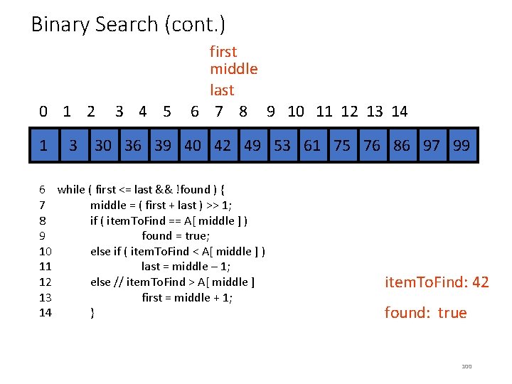
Binary Search (cont. ) 0 1 2 3 4 5 first middle last 6 7 8 9 10 11 12 13 14 34 1 34 3 30 36 39 40 42 34 49 34 53 61 75 76 86 97 99 6 while ( first <= last && !found ) { 7 middle = ( first + last ) >> 1; 8 9 10 11 12 13 14 if ( item. To. Find == A[ middle ] ) found = true; else if ( item. To. Find < A[ middle ] ) last = middle – 1; else // item. To. Find > A[ middle ] first = middle + 1; } item. To. Find: 42 found: true 98

Binary Search (cont. ) 0 1 2 3 4 5 first middle last 6 7 8 9 10 11 12 13 14 34 1 34 3 30 36 39 40 42 34 49 34 53 61 75 76 86 97 99 6 while ( first <= last && !found ) { 7 8 9 10 11 12 13 14 middle = ( first + last ) >> 1; if ( item. To. Find == A[ middle ] ) found = true; else if ( item. To. Find < A[ middle ] ) last = middle – 1; else // item. To. Find > A[ middle ] first = middle + 1; } item. To. Find: 42 found: true 99

Binary Search (cont. ) 0 1 2 3 4 5 first middle last 6 7 8 9 10 11 12 13 14 34 1 34 3 30 36 39 40 42 34 49 34 53 61 75 76 86 97 99 6 while ( first <= last && !found ) { 7 middle = ( first + last ) >> 1; 8 if ( item. To. Find == A[ middle ] ) 9 found = true; 10 else if ( item. To. Find < A[ middle ] ) 11 last = middle – 1; 12 else // item. To. Find > A[ middle ] 13 first = middle + 1; 14 } item. To. Find: 42 found: true 100

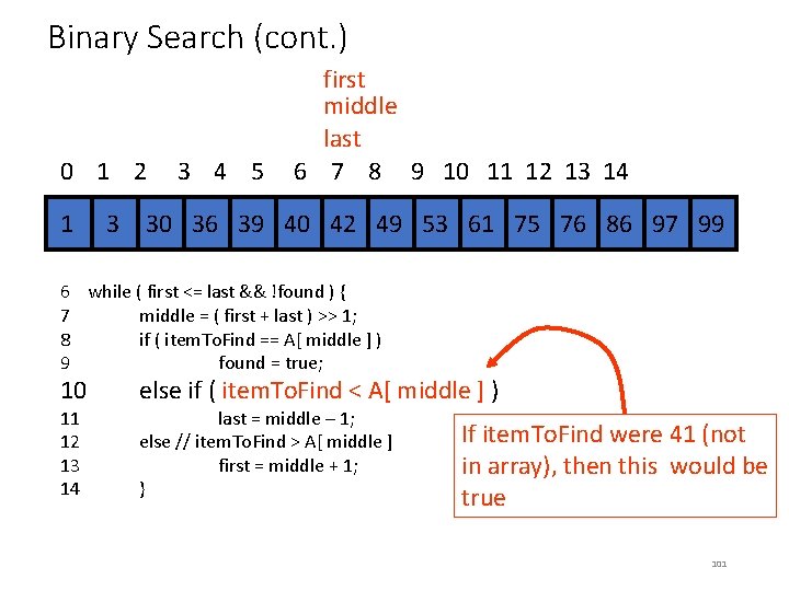
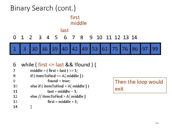
Binary Search (cont. ) 0 1 2 3 4 5 first middle last 6 7 8 9 10 11 12 13 14 34 1 34 3 30 36 39 40 42 34 49 34 53 61 75 76 86 97 99 6 while ( first <= last && !found ) { 7 middle = ( first + last ) >> 1; 8 if ( item. To. Find == A[ middle ] ) 9 found = true; 10 11 12 13 14 else if ( item. To. Find < A[ middle ] ) last = middle – 1; else // item. To. Find > A[ middle ] first = middle + 1; } If item. To. Find were 41 (not in array), then this would be true 101

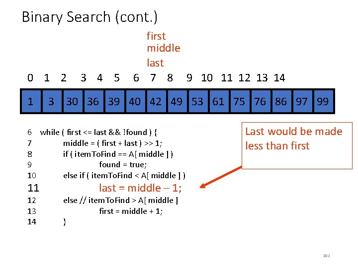
Binary Search (cont. ) 0 1 2 3 4 5 first middle last 6 7 8 9 10 11 12 13 14 34 1 34 3 30 36 39 40 42 34 49 34 53 61 75 76 86 97 99 6 while ( first <= last && !found ) { 7 middle = ( first + last ) >> 1; 8 if ( item. To. Find == A[ middle ] ) 9 found = true; 10 else if ( item. To. Find < A[ middle ] ) 11 12 13 14 Last would be made less than first last = middle – 1; else // item. To. Find > A[ middle ] first = middle + 1; } 102

Binary Search (cont. ) first middle 0 1 2 last 3 4 5 6 7 8 9 10 11 12 13 14 34 1 34 3 30 36 39 40 42 34 49 34 53 61 75 76 86 97 99 6 while ( first <= last && !found ) { 7 middle = ( first + last ) >> 1; 8 if ( item. To. Find == A[ middle ] ) 9 found = true; 10 else if ( item. To. Find < A[ middle ] ) 11 12 13 14 Last would be made less than first last = middle – 1; else // item. To. Find > A[ middle ] first = middle + 1; } 103

Binary Search (cont. ) first middle 0 1 2 last 3 4 5 6 7 8 9 10 11 12 13 14 34 1 34 3 30 36 39 40 42 34 49 34 53 61 75 76 86 97 99 6 while ( first <= last && !found ) { 7 8 9 10 11 12 13 14 middle = ( first + last ) >> 1; if ( item. To. Find == A[ middle ] ) found = true; else if ( item. To. Find < A[ middle ] ) last = middle – 1; else // item. To. Find > A[ middle ] first = middle + 1; } Then the loop would exit 104

Binary Search (cont. ) 1 2 3 4 5 6 7 8 9 10 11 12 13 14 int first = 0; int last = size – 1; int middle; bool found = false; Overloaded operators when templated while ( first <= last && !found ) { middle = ( first + last ) >> 1; if ( item. To. Find == A[ middle ] ) found = true; else if ( item. To. Find < A[ middle ] ) last = middle – 1; else // item. To. Find > A[ middle ] first = middle + 1; } 105

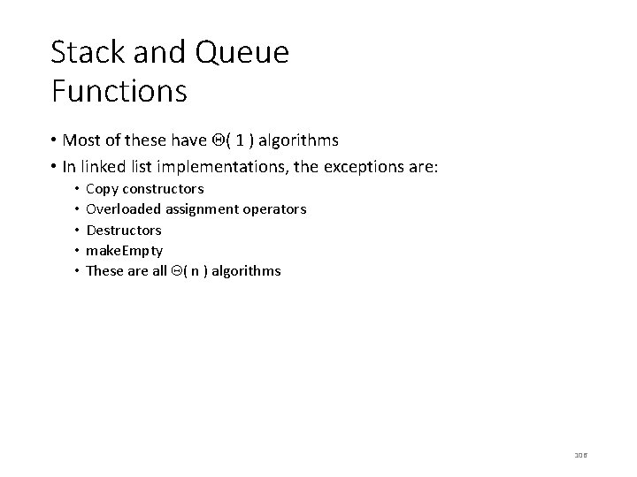
Stack and Queue Functions • Most of these have ( 1 ) algorithms • In linked list implementations, the exceptions are: • • • Copy constructors Overloaded assignment operators Destructors make. Empty These are all ( n ) algorithms 106

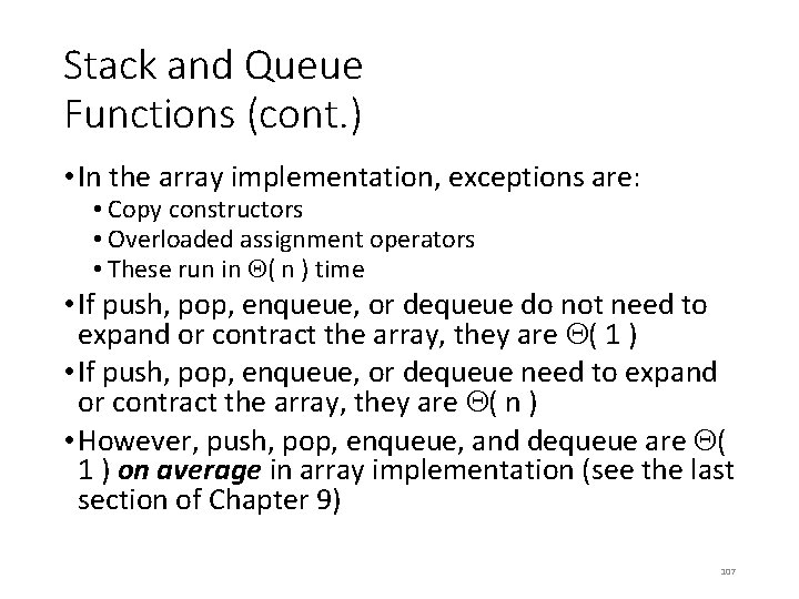
Stack and Queue Functions (cont. ) • In the array implementation, exceptions are: • Copy constructors • Overloaded assignment operators • These run in ( n ) time • If push, pop, enqueue, or dequeue do not need to expand or contract the array, they are ( 1 ) • If push, pop, enqueue, or dequeue need to expand or contract the array, they are ( n ) • However, push, pop, enqueue, and dequeue are ( 1 ) on average in array implementation (see the last section of Chapter 9) 107

ALGORITHM ANALYSIS • Analysis of Resource consumption by processor • • Time Memory Number of processors Power 108

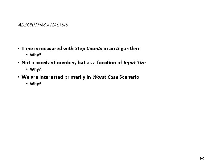
ALGORITHM ANALYSIS • Time is measured with Step Counts in an Algorithm • Why? • Not a constant number, but as a function of Input Size • Why? • We are interested primarily in Worst Case Scenario: • Why? 109

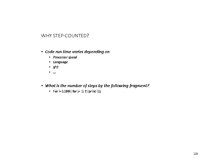
WHY STEP-COUNTED? • Code run time varies depending on • • Processor speed Language I/O … • What is the number of steps by the following fragment? • For i=1: 100 { for j= 1: 2 {print i}}; 110

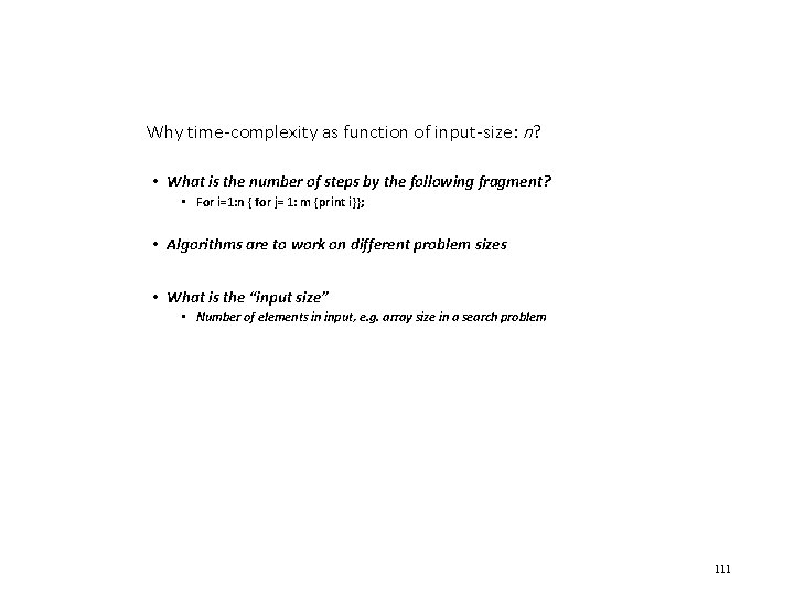
Why time-complexity as function of input-size: n? • What is the number of steps by the following fragment? • For i=1: n { for j= 1: m {print i}}; • Algorithms are to work on different problem sizes • What is the “input size” • Number of elements in input, e. g. array size in a search problem 111

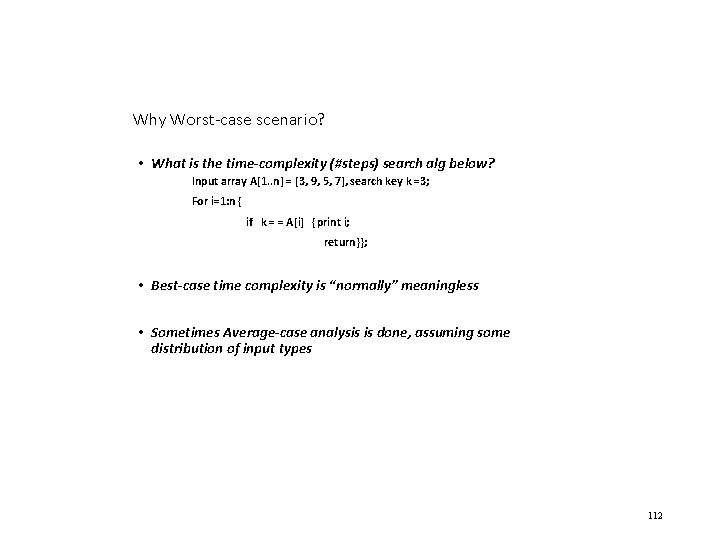
Why Worst-case scenario? • What is the time-complexity (#steps) search alg below? Input array A[1. . n] = [3, 9, 5, 7], search key k =3; For i=1: n { if k = = A[i] {print i; return}}; • Best-case time complexity is “normally” meaningless • Sometimes Average-case analysis is done, assuming some distribution of input types 112

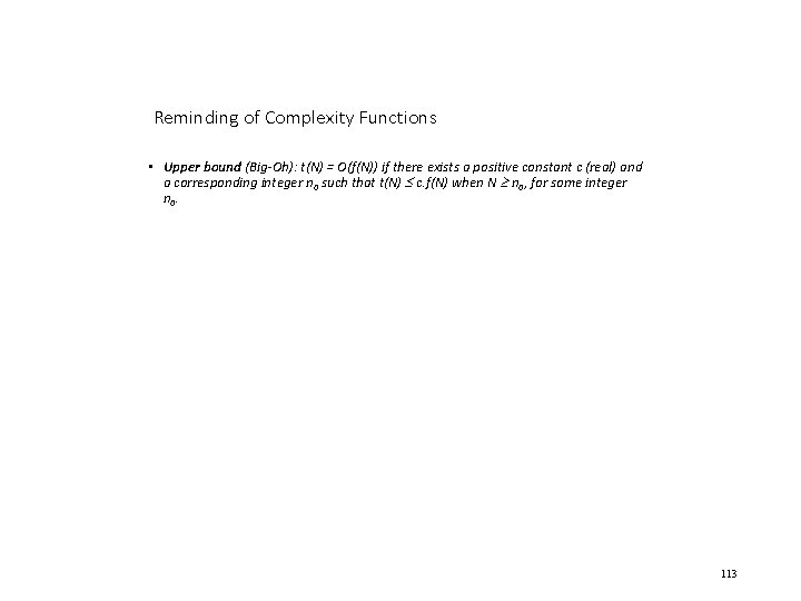
Reminding of Complexity Functions • Upper bound (Big-Oh): t(N) = O(f(N)) if there exists a positive constant c (real) and a corresponding integer n 0 such that t(N) c. f(N) when N n 0, for some integer n 0. 113

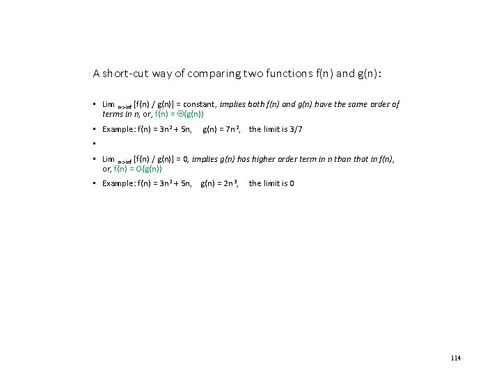
A short-cut way of comparing two functions f(n) and g(n): • Lim n->inf [f(n) / g(n)] = constant, implies both f(n) and g(n) have the same order of terms in n, or, f(n) = (g(n)) • Example: f(n) = 3 n 2 + 5 n, g(n) = 7 n 2, the limit is 3/7 • • Lim n->inf [f(n) / g(n)] = 0, implies g(n) has higher order term in n that in f(n), or, f(n) = O(g(n)) • Example: f(n) = 3 n 2 + 5 n, g(n) = 2 n 3, the limit is 0 114

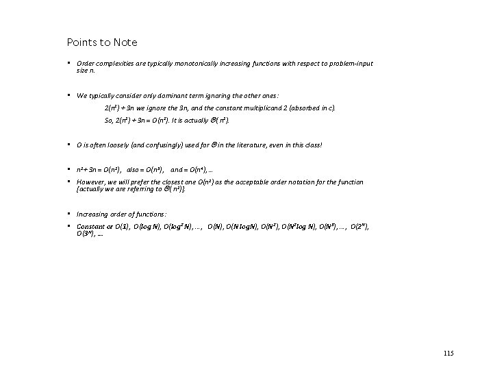
Points to Note • Order complexities are typically monotonically increasing functions with respect to problem-input size n. • We typically consider only dominant term ignoring the other ones: 2(n 2) + 3 n we ignore the 3 n, and the constant multiplicand 2 (absorbed in c). So, 2(n 2) + 3 n = O(n 2). It is actually ( n 2). • O is often loosely (and confusingly) used for in the literature, even in this class! • n 2+ 3 n = O(n 2), also = O(n 3), and = O(n 4), … • However, we will prefer the closest one O(n 2) as the acceptable order notation for the function [actually we are referring to ( n 2)]. • Increasing order of functions: • Constant or O(1), O(log N), O(log 2 N), …, O(N), O(N log. N), O(N 2 log N), O(N 3), …, O(2 N), O(3 N), … 115

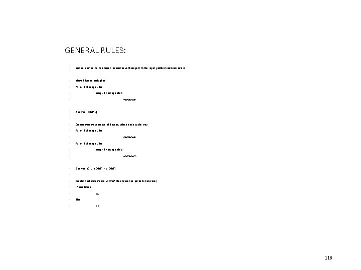
GENERAL RULES: • Loops: number of iterations/ recursions with respect to the input problem instance size N • Nested loops: multiplied • for I = 1 through N do • for j = 1 through N do • • -whatever- Analysis: O(N*N) • • Consecutive statements: add steps, which leads to the max • for I = 1 through N do • • -whateverfor I = 1 through N do • for j = 1 through N do • • -moreover- Analysis: O(N) + O(N 2) --> O(N 2) • • Conditional statements: max of the alternative paths (worst-case) • If (condition) • • • S 1 Else S 2 116

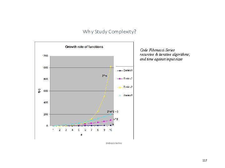
Why Study Complexity? Code Fibonacci Series recursive & iterative algorithms; and time against input sizes Debasis Mitra 117

Background Needed • Data Structures: Big-O notations, Linked list, Sorting, Searching, recursion, , , • Discrete Mathematics: Set theory, Logic, Recurrence equation, Matrix operations, , , • Programming experience 118

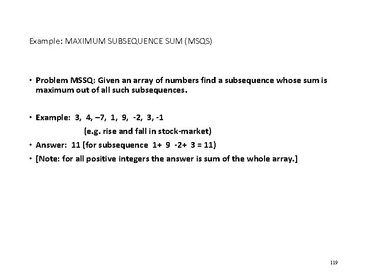
Example: MAXIMUM SUBSEQUENCE SUM (MSQS) • Problem MSSQ: Given an array of numbers find a subsequence whose sum is maximum out of all such subsequences. • Example: 3, 4, – 7, 1, 9, -2, 3, -1 (e. g. rise and fall in stock-market) • Answer: 11 (for subsequence 1+ 9 -2+ 3 = 11) • [Note: for all positive integers the answer is sum of the whole array. ] 119

MSQS Algorithm 1 • Input: Array A[N], e. g. [3, 4, – 7, 1, 9, -2, 3, -1 ] • Output: Maximum subsequence sum, e. g. , 11 • Algorithm 1: 1. max. Sum = 0; // We expect non-negative value here at the end 2. for (i = 0 through N-1) do 3. for (j = i through N-1) do // choice of subsequence i through j 4. { this. Sum = 0; 5. for (k = i through j) do // addition loop 6. this. Sum = this. Sum + a[k]; // O(N 3) 7. 8. if (this. Sum > max. Sum) then 9. max. Sum = this. Sum; // O(N 2) 10. } 11. return max. Sum; End Algorithm 1. • Analysis of Algorithm 1: i=0 N-1 j=i. N-1 k=ij 1 = … = O(N 3) 120

MSQS Algorithm 2 • Input: Array A[N], e. g. [3, 4, – 7, 1, 9, -2, 3, -1 ] • Output: Maximum subsequence sum, e. g. , 11 • Algorithm 2: 1. max. Sum = 0; // We expect non-negative value here at the end 2. for (i = 0 through N-1) do 3. this. Sum = 0; 4. for (j = i through N-1) do 5. { this. Sum = this. Sum + a[j]; // reuse the partial sum from 6. // the previous iteration 7. if (this. Sum > max. Sum) then 8. max. Sum = this. Sum; 9. } 10. return max. Sum; • End Algorithm 2. • Analysis of Algorithm 2: i=0 N-1 j=i. N-1 1 = … = O(N 2) 121

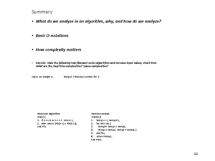
Summary • What do we analyze in an algorithm, why, and how do we analyze? • Basic O-notations • How complexity matters • Exercise: Code the following two fibonacci series algorithms and increase input values, check time. What are the step/time-complexities? Space-complexities? Input: an integer n; Output: Fibonacci number for n Recursive Algorithm: Fib(n) { 1. if n = = 0 or n = = 1 return 1; 2. else return (Fib(n-1) + Fib(n-2)); End Fib. Iterative version: Fib. It(n) { 1. temp 1 = 1; temp 2=1; 2. for i=3: n do { 3. temp 3 = temp 1 + temp 2; 4. temp 1 = temp 2; temp 2 = temp 3; } 5. end for; 6. return temp 2; End Fib. It. 122