C 280 Computer Vision Prof Trevor Darrell trevoreecs

C 280, Computer Vision Prof. Trevor Darrell trevor@eecs. berkeley. edu Lecture 2: Image Formation

Administrivia • • • We’re now in 405 Soda… New office hours: Thurs. 5 -6 pm, 413 Soda. I’ll decide on waitlist decisions tomorrow. Any Matlab issues yet? Roster…

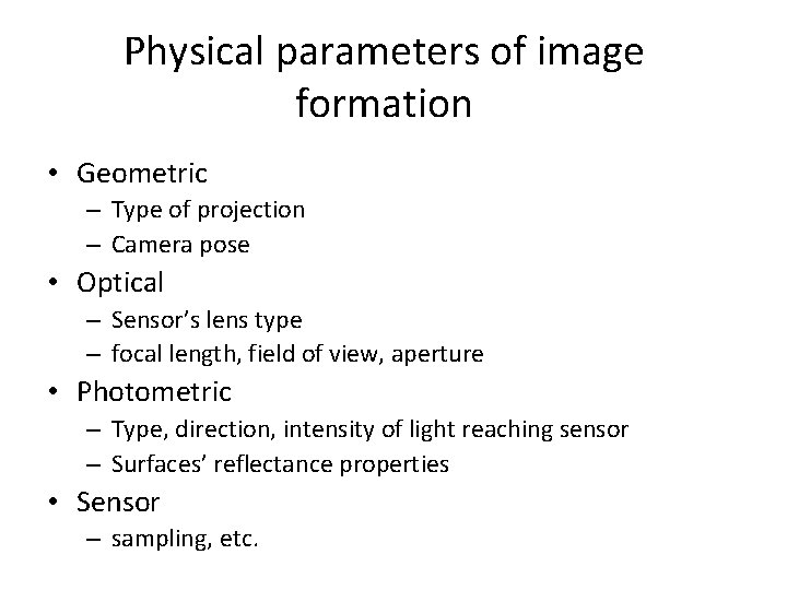
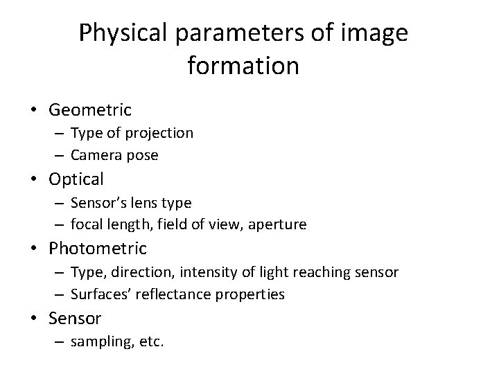
Physical parameters of image formation • Geometric – Type of projection – Camera pose • Optical – Sensor’s lens type – focal length, field of view, aperture • Photometric – Type, direction, intensity of light reaching sensor – Surfaces’ reflectance properties • Sensor – sampling, etc.

Physical parameters of image formation • Geometric – Type of projection – Camera pose • Optical – Sensor’s lens type – focal length, field of view, aperture • Photometric – Type, direction, intensity of light reaching sensor – Surfaces’ reflectance properties • Sensor – sampling, etc.

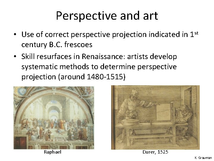
Perspective and art • Use of correct perspective projection indicated in 1 st century B. C. frescoes • Skill resurfaces in Renaissance: artists develop systematic methods to determine perspective projection (around 1480 -1515) Raphael Durer, 1525 K. Grauman

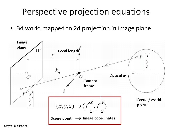
Perspective projection equations • 3 d world mapped to 2 d projection in image plane Image plane Focal length Optical axis Camera frame ‘’ Scene point Forsyth and Ponce ‘ ’ Image coordinates Scene / world points

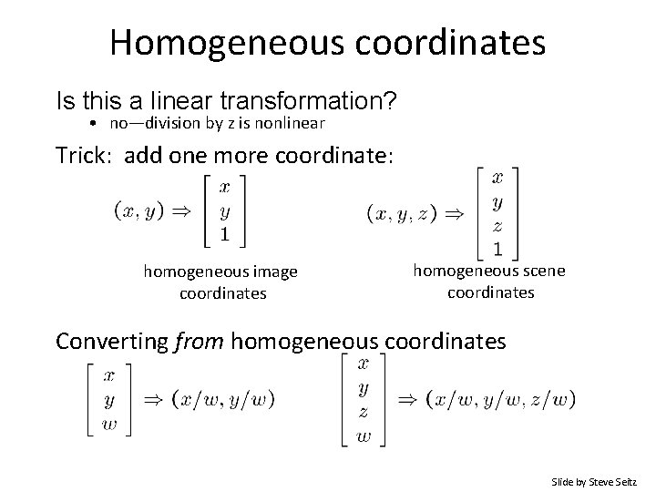
Homogeneous coordinates Is this a linear transformation? • no—division by z is nonlinear Trick: add one more coordinate: homogeneous image coordinates homogeneous scene coordinates Converting from homogeneous coordinates Slide by Steve Seitz

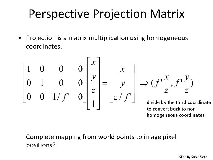
Perspective Projection Matrix • Projection is a matrix multiplication using homogeneous coordinates: divide by the third coordinate to convert back to nonhomogeneous coordinates Complete mapping from world points to image pixel positions? Slide by Steve Seitz

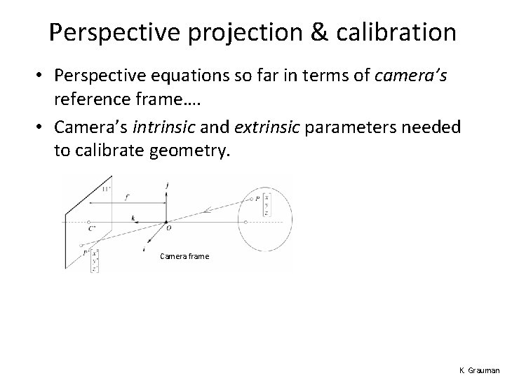
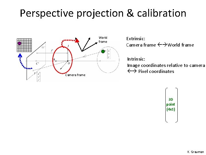
Perspective projection & calibration • Perspective equations so far in terms of camera’s reference frame…. • Camera’s intrinsic and extrinsic parameters needed to calibrate geometry. Camera frame K. Grauman

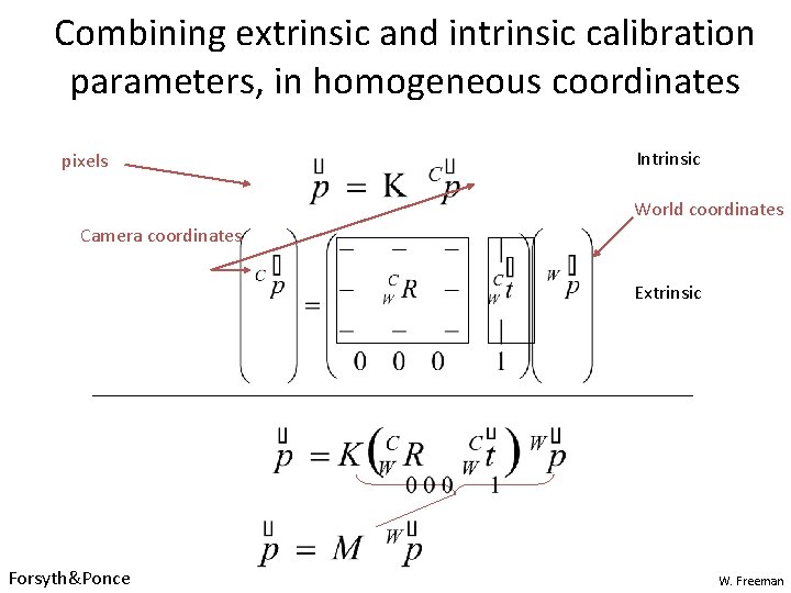
Perspective projection & calibration World frame Intrinsic: Image coordinates relative to camera Pixel coordinates Camera frame 2 D point (3 x 1) = Camera to pixel coord. trans. matrix (3 x 3) Extrinsic: Camera frame World frame Perspective projection matrix (3 x 4) World to camera coord. trans. matrix (4 x 4) 3 D point (4 x 1) K. Grauman

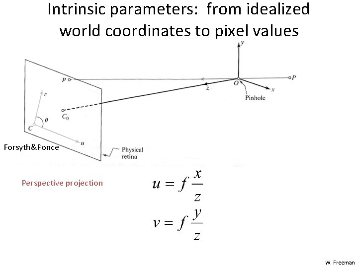
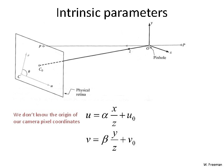
Intrinsic parameters: from idealized world coordinates to pixel values Forsyth&Ponce Perspective projection W. Freeman

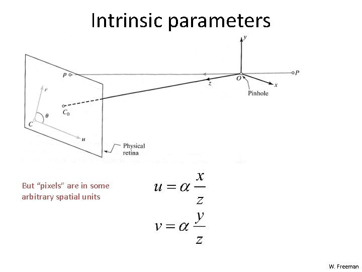
Intrinsic parameters But “pixels” are in some arbitrary spatial units W. Freeman

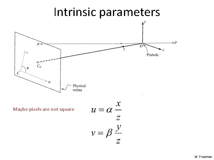
Intrinsic parameters Maybe pixels are not square W. Freeman

Intrinsic parameters We don’t know the origin of our camera pixel coordinates W. Freeman

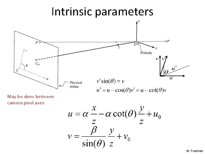
Intrinsic parameters May be skew between camera pixel axes W. Freeman

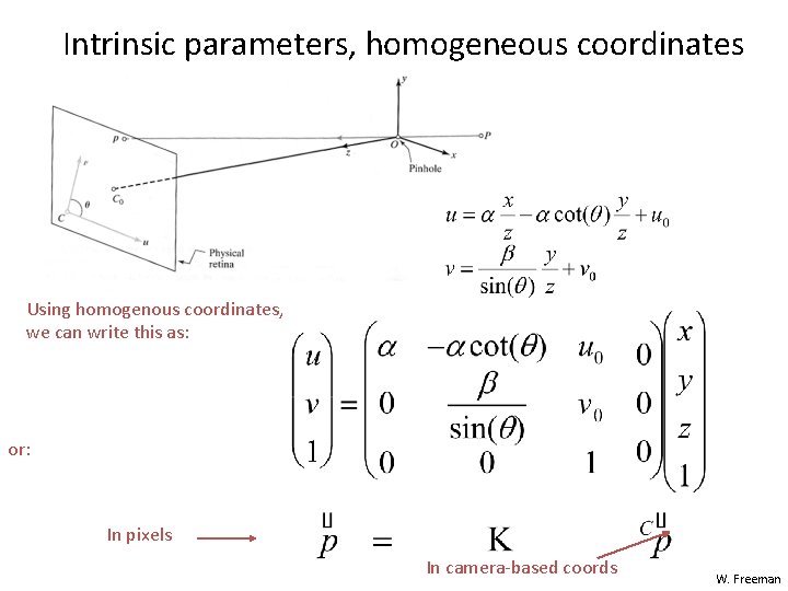
Intrinsic parameters, homogeneous coordinates Using homogenous coordinates, we can write this as: or: In pixels In camera-based coords W. Freeman

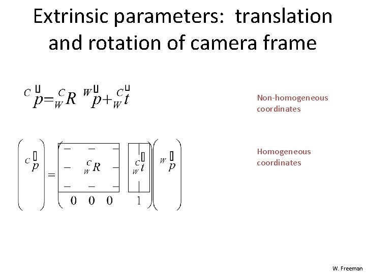
Extrinsic parameters: translation and rotation of camera frame Non-homogeneous coordinates Homogeneous coordinates W. Freeman

Combining extrinsic and intrinsic calibration parameters, in homogeneous coordinates pixels Intrinsic World coordinates Camera coordinates Extrinsic Forsyth&Ponce W. Freeman

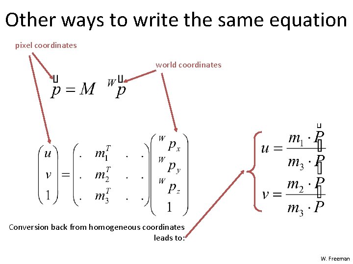
Other ways to write the same equation pixel coordinates world coordinates Conversion back from homogeneous coordinates leads to: W. Freeman

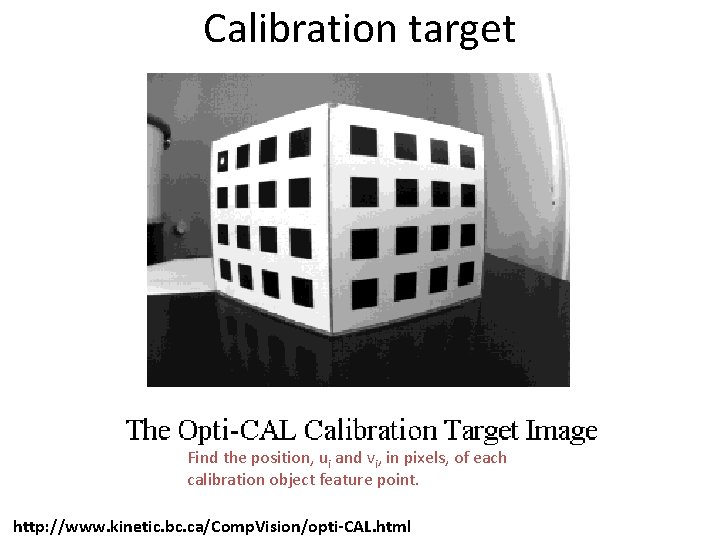
Calibration target Find the position, ui and vi, in pixels, of each calibration object feature point. http: //www. kinetic. bc. ca/Comp. Vision/opti-CAL. html

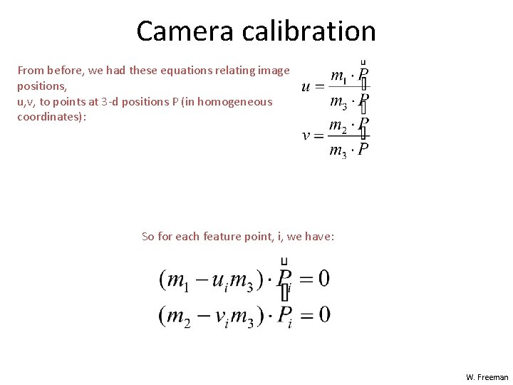
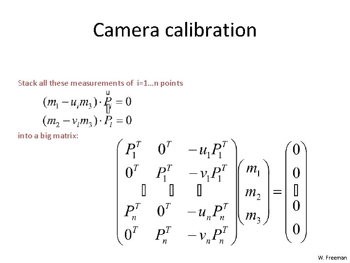
Camera calibration From before, we had these equations relating image positions, u, v, to points at 3 -d positions P (in homogeneous coordinates): So for each feature point, i, we have: W. Freeman

Camera calibration Stack all these measurements of i=1…n points into a big matrix: W. Freeman

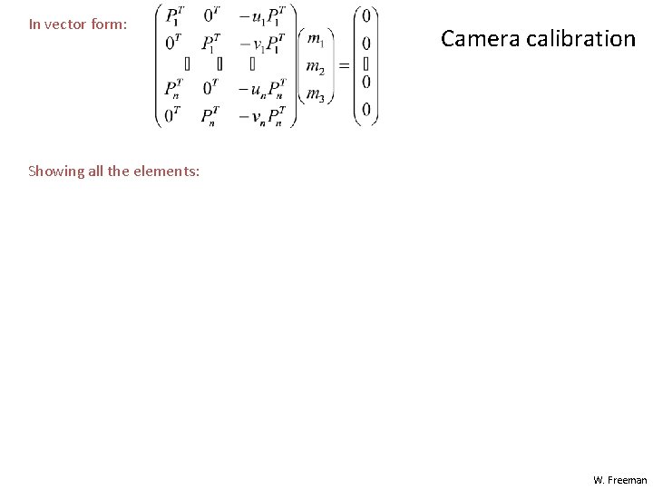
In vector form: Camera calibration Showing all the elements: W. Freeman

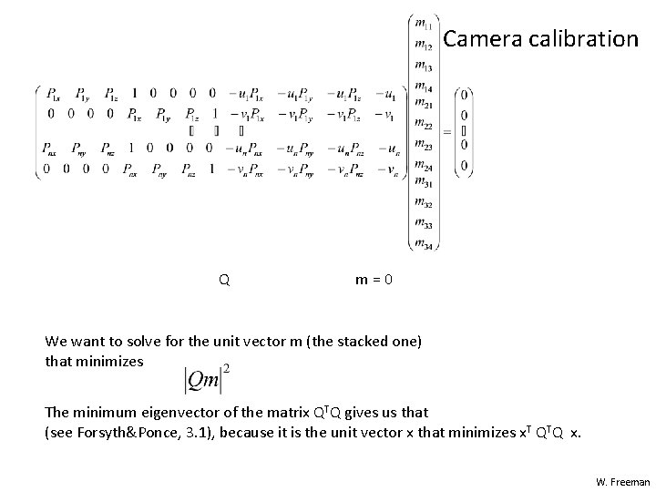
Camera calibration Q m = 0 We want to solve for the unit vector m (the stacked one) that minimizes The minimum eigenvector of the matrix QTQ gives us that (see Forsyth&Ponce, 3. 1), because it is the unit vector x that minimizes x T QTQ x. W. Freeman

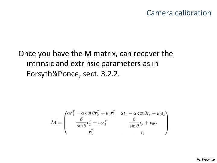
Camera calibration Once you have the M matrix, can recover the intrinsic and extrinsic parameters as in Forsyth&Ponce, sect. 3. 2. 2. W. Freeman

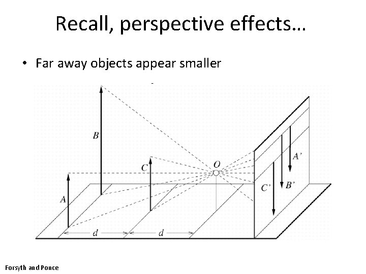
Recall, perspective effects… • Far away objects appear smaller Forsyth and Ponce

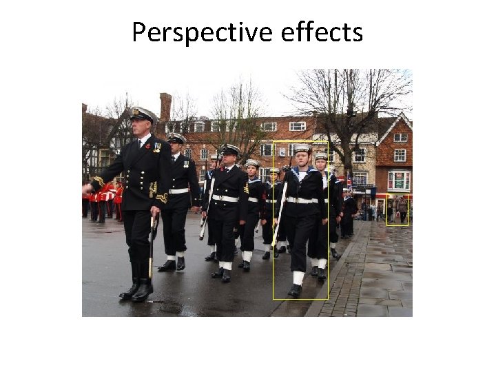
Perspective effects

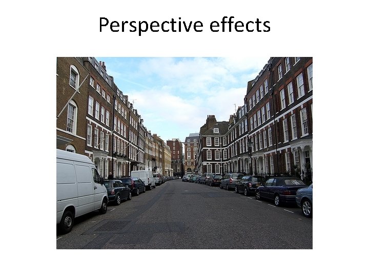
Perspective effects

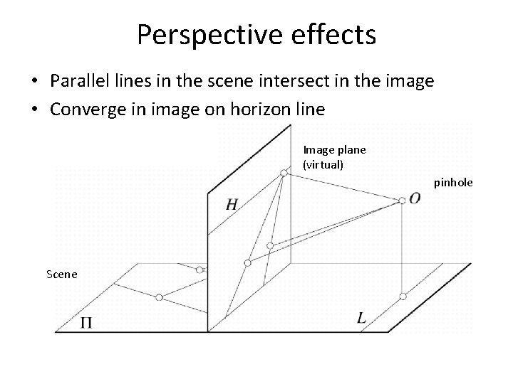
Perspective effects • Parallel lines in the scene intersect in the image • Converge in image on horizon line Image plane (virtual) pinhole Scene

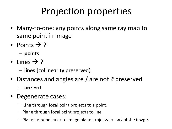
Projection properties • Many-to-one: any points along same ray map to same point in image • Points ? – points • Lines ? – lines (collinearity preserved) • Distances and angles are / are not ? preserved – are not • Degenerate cases: – Line through focal point projects to a point. – Plane through focal point projects to line – Plane perpendicular to image plane projects to part of the image.

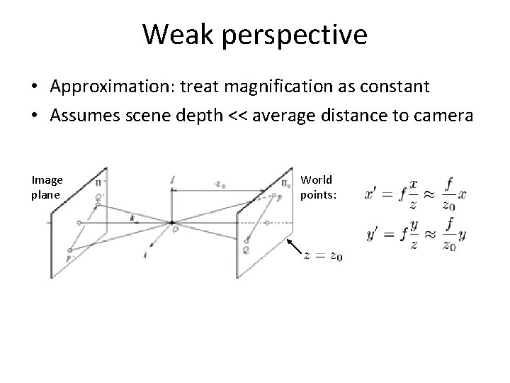
Weak perspective • Approximation: treat magnification as constant • Assumes scene depth << average distance to camera Image plane World points:

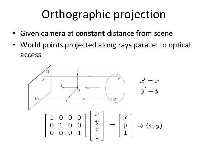
Orthographic projection • Given camera at constant distance from scene • World points projected along rays parallel to optical access

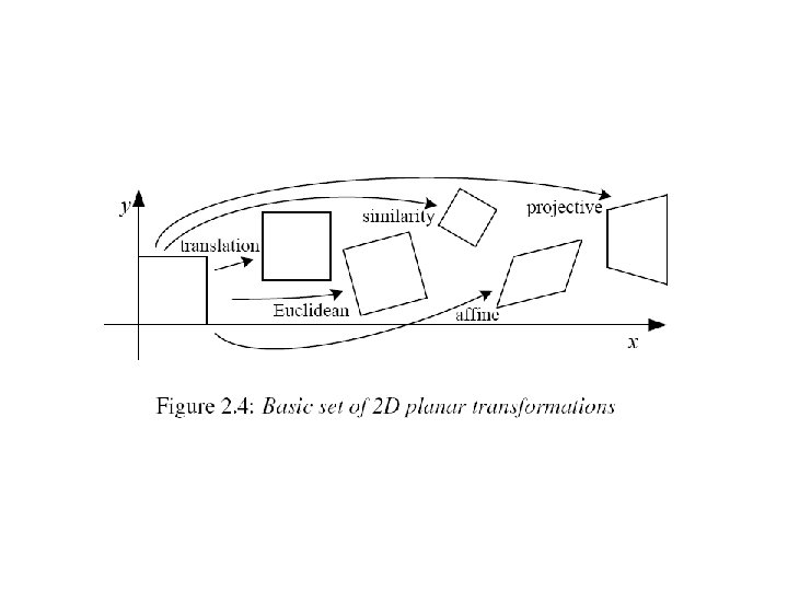
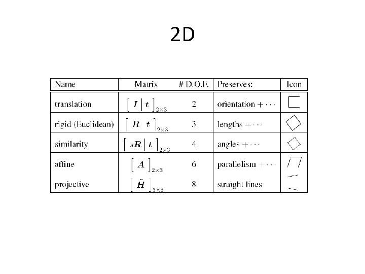
2 D

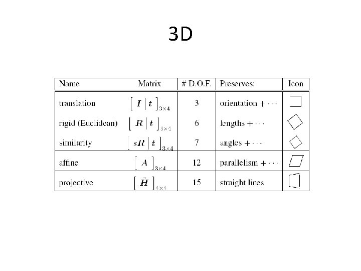
3 D

Other types of projection • Lots of intriguing variants… • (I’ll just mention a few fun ones) S. Seitz

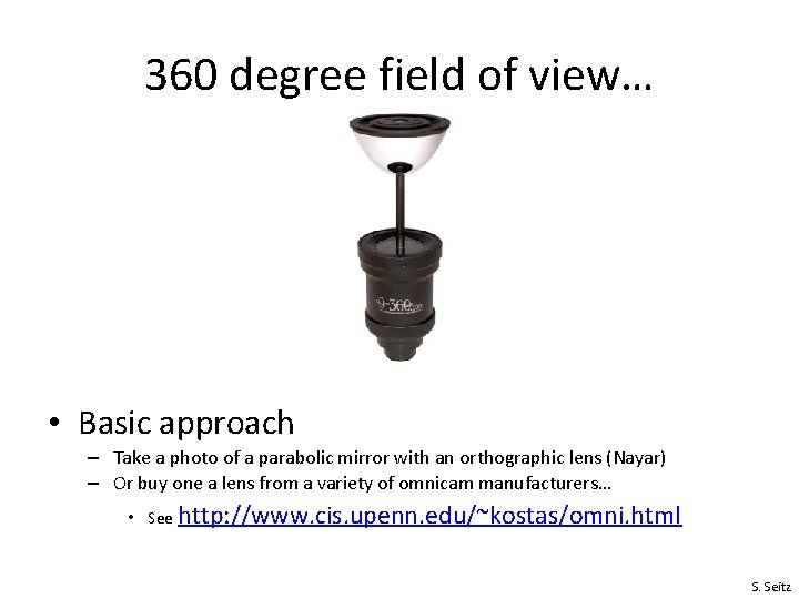
360 degree field of view… • Basic approach – Take a photo of a parabolic mirror with an orthographic lens (Nayar) – Or buy one a lens from a variety of omnicam manufacturers… • See http: //www. cis. upenn. edu/~kostas/omni. html S. Seitz

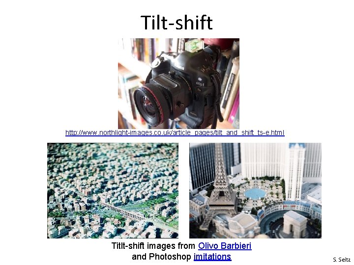
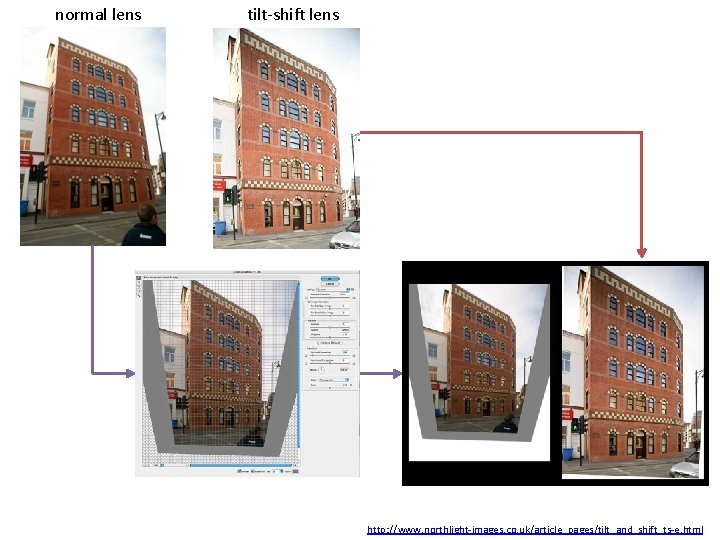
Tilt-shift http: //www. northlight-images. co. uk/article_pages/tilt_and_shift_ts-e. html Titlt-shift images from Olivo Barbieri and Photoshop imitations S. Seitz

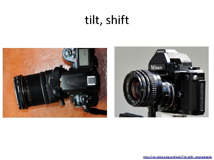
tilt, shift http: //en. wikipedia. org/wiki/Tilt-shift_photography

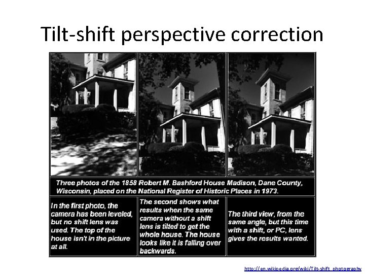
Tilt-shift perspective correction http: //en. wikipedia. org/wiki/Tilt-shift_photography

normal lens tilt-shift lens http: //www. northlight-images. co. uk/article_pages/tilt_and_shift_ts-e. html

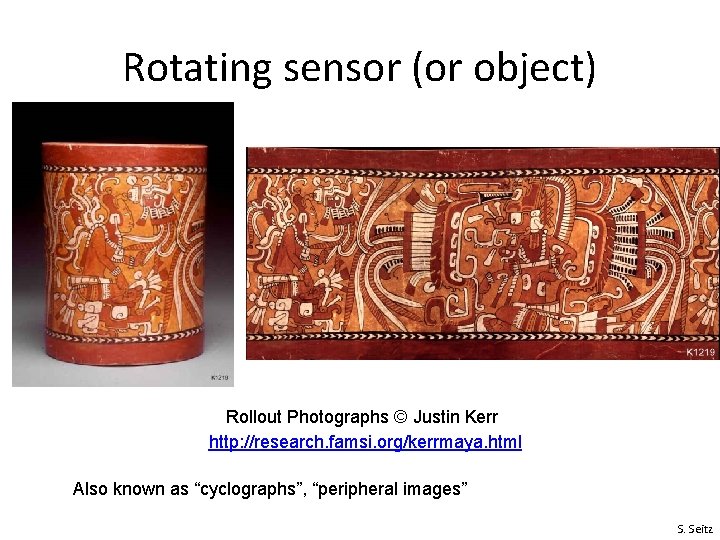
Rotating sensor (or object) Rollout Photographs © Justin Kerr http: //research. famsi. org/kerrmaya. html Also known as “cyclographs”, “peripheral images” S. Seitz

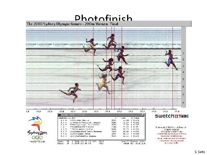
Photofinish S. Seitz

Physical parameters of image formation • Geometric – Type of projection – Camera pose • Optical – Sensor’s lens type – focal length, field of view, aperture • Photometric – Type, direction, intensity of light reaching sensor – Surfaces’ reflectance properties • Sensor – sampling, etc.

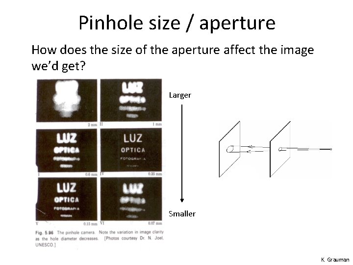
Pinhole size / aperture How does the size of the aperture affect the image we’d get? Larger Smaller K. Grauman

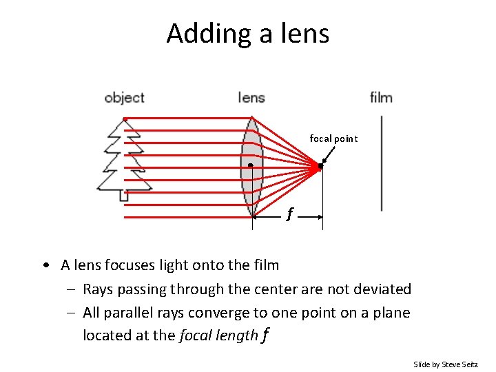
Adding a lens focal point f • A lens focuses light onto the film – Rays passing through the center are not deviated – All parallel rays converge to one point on a plane located at the focal length f Slide by Steve Seitz

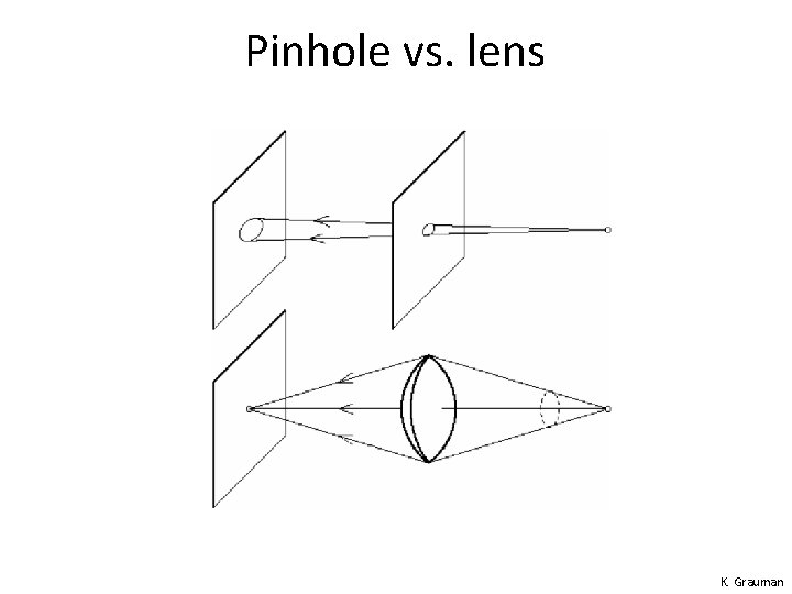
Pinhole vs. lens K. Grauman

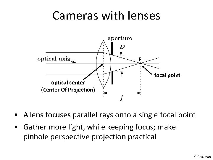
Cameras with lenses F focal point optical center (Center Of Projection) • A lens focuses parallel rays onto a single focal point • Gather more light, while keeping focus; make pinhole perspective projection practical K. Grauman

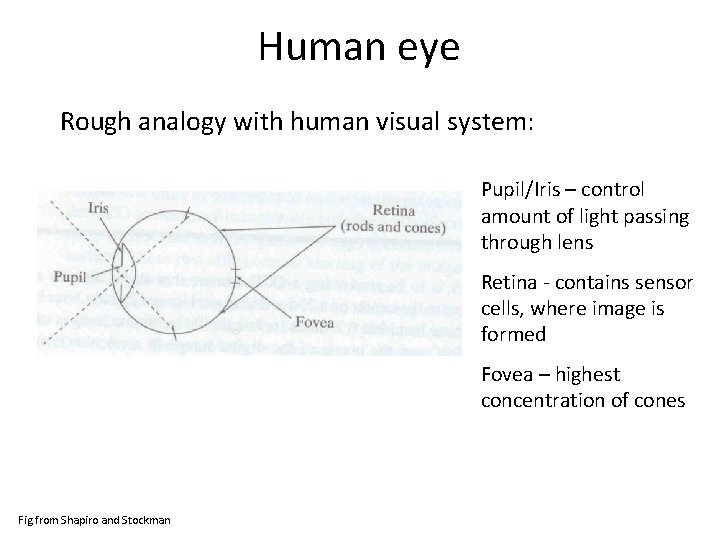
Human eye Rough analogy with human visual system: Pupil/Iris – control amount of light passing through lens Retina - contains sensor cells, where image is formed Fovea – highest concentration of cones Fig from Shapiro and Stockman

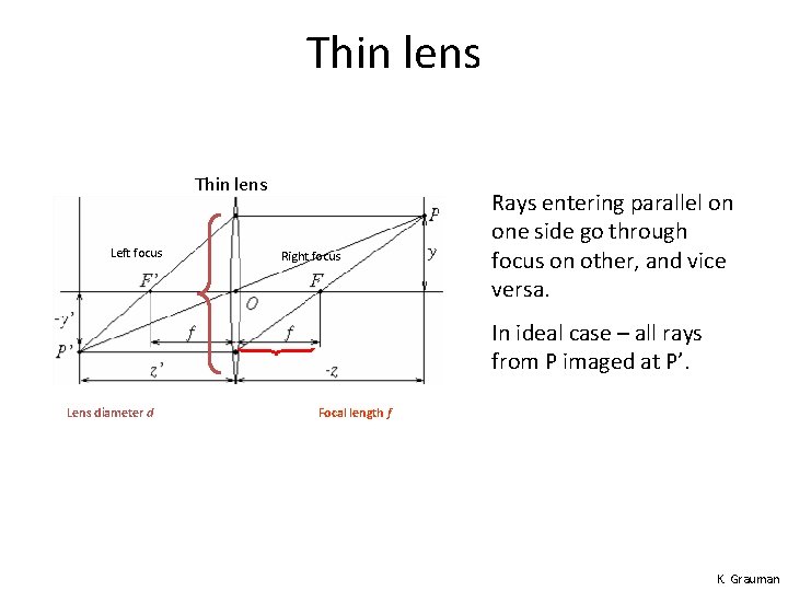
Thin lens Left focus Right focus Rays entering parallel on one side go through focus on other, and vice versa. In ideal case – all rays from P imaged at P’. Lens diameter d Focal length f K. Grauman

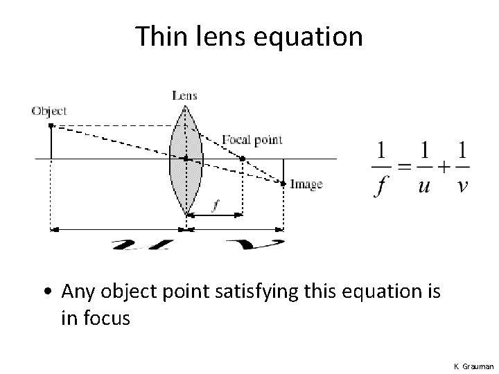
Thin lens equation • Any object point satisfying this equation is in focus K. Grauman

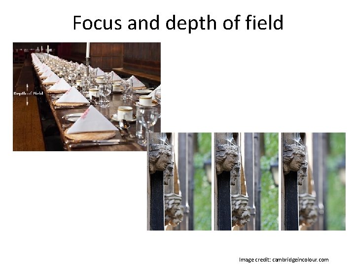
Focus and depth of field Image credit: cambridgeincolour. com

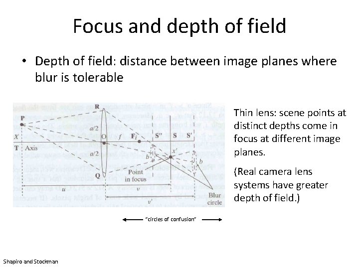
Focus and depth of field • Depth of field: distance between image planes where blur is tolerable Thin lens: scene points at distinct depths come in focus at different image planes. (Real camera lens systems have greater depth of field. ) “circles of confusion” Shapiro and Stockman

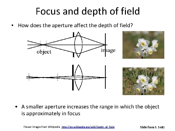
Focus and depth of field • How does the aperture affect the depth of field? • A smaller aperture increases the range in which the object is approximately in focus Flower images from Wikipedia http: //en. wikipedia. org/wiki/Depth_of_field Slide from S. Seitz

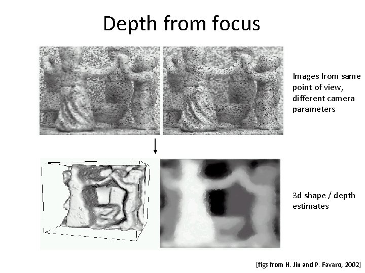
Depth from focus Images from same point of view, different camera parameters 3 d shape / depth estimates [figs from H. Jin and P. Favaro, 2002]

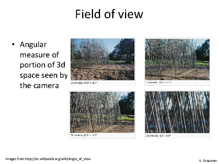
Field of view • Angular measure of portion of 3 d space seen by the camera Images from http: //en. wikipedia. org/wiki/Angle_of_view K. Grauman

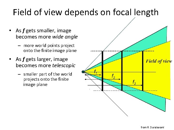
Field of view depends on focal length • As f gets smaller, image becomes more wide angle – more world points project onto the finite image plane • As f gets larger, image becomes more telescopic – smaller part of the world projects onto the finite image plane from R. Duraiswami

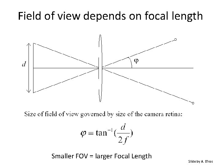
Field of view depends on focal length Smaller FOV = larger Focal Length Slide by A. Efros

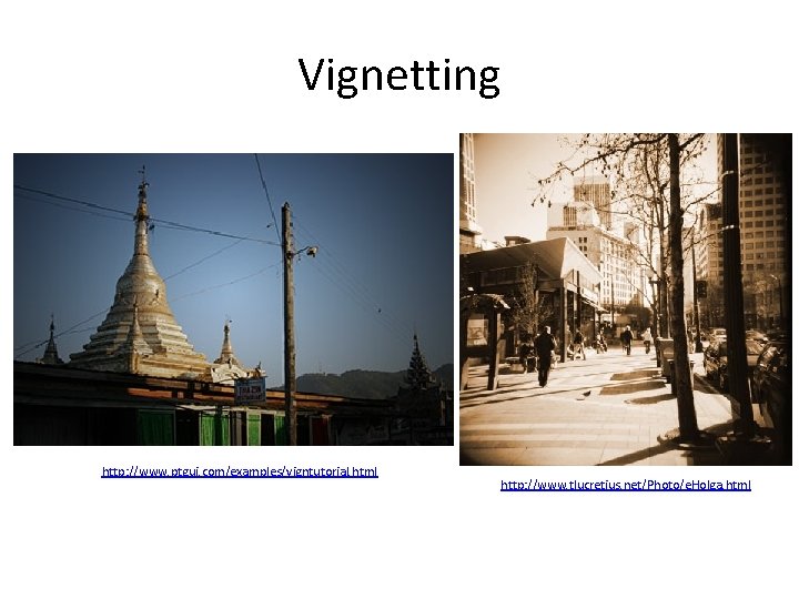
Vignetting http: //www. ptgui. com/examples/vigntutorial. html http: //www. tlucretius. net/Photo/e. Holga. html

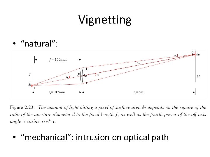
Vignetting • “natural”: • “mechanical”: intrusion on optical path

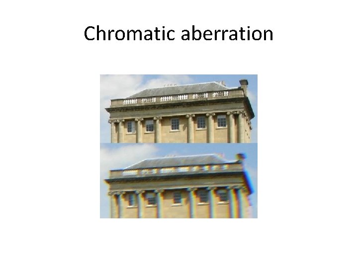
Chromatic aberration

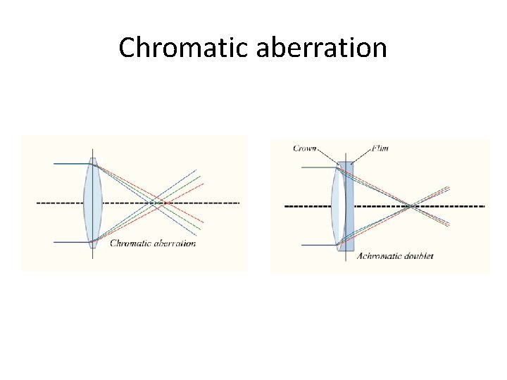
Chromatic aberration

Physical parameters of image formation • Geometric – Type of projection – Camera pose • Optical – Sensor’s lens type – focal length, field of view, aperture • Photometric – Type, direction, intensity of light reaching sensor – Surfaces’ reflectance properties • Sensor – sampling, etc.

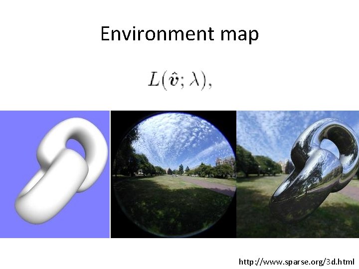
Environment map http: //www. sparse. org/3 d. html

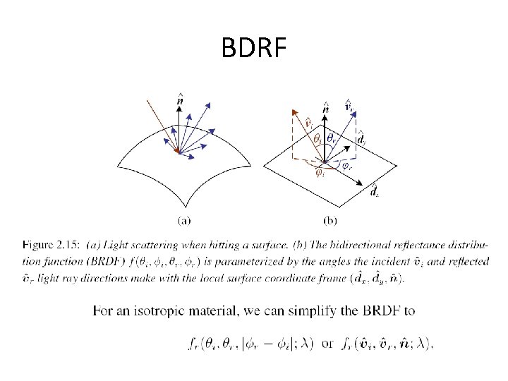
BDRF

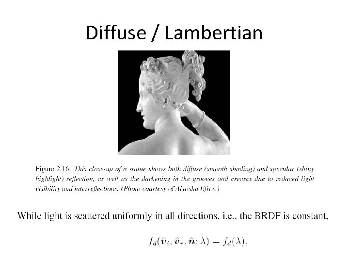
Diffuse / Lambertian

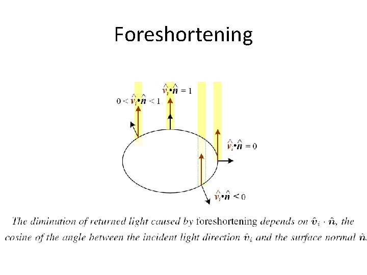
Foreshortening

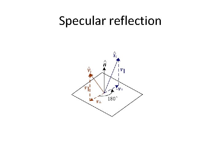
Specular reflection

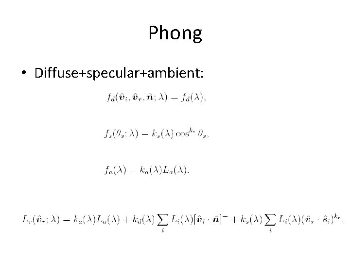
Phong • Diffuse+specular+ambient:

Physical parameters of image formation • Geometric – Type of projection – Camera pose • Optical – Sensor’s lens type – focal length, field of view, aperture • Photometric – Type, direction, intensity of light reaching sensor – Surfaces’ reflectance properties • Sensor – sampling, etc.

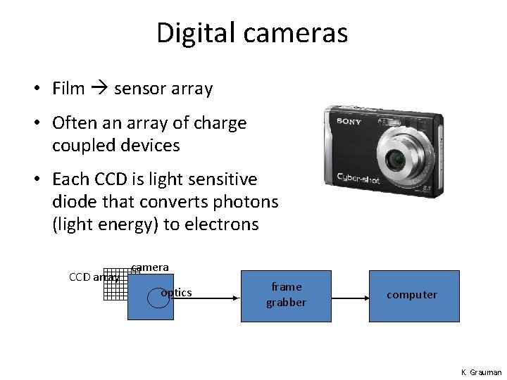
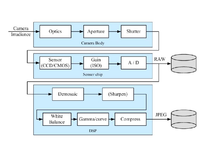
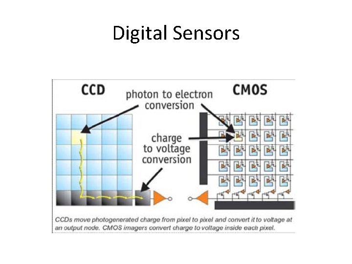
Digital cameras • Film sensor array • Often an array of charge coupled devices • Each CCD is light sensitive diode that converts photons (light energy) to electrons CCD array camera optics frame grabber computer K. Grauman

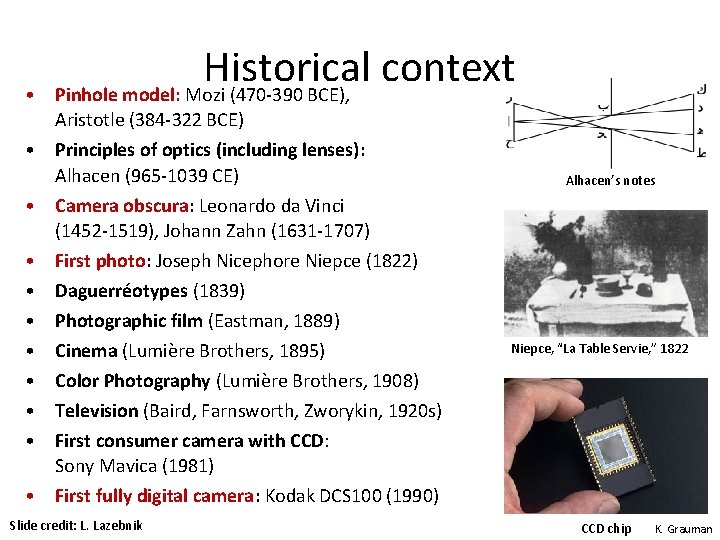
• Historical context Pinhole model: Mozi (470 -390 BCE), Aristotle (384 -322 BCE) • Principles of optics (including lenses): Alhacen (965 -1039 CE) • Camera obscura: Leonardo da Vinci (1452 -1519), Johann Zahn (1631 -1707) • • First photo: Joseph Nicephore Niepce (1822) Daguerréotypes (1839) Photographic film (Eastman, 1889) Cinema (Lumière Brothers, 1895) Color Photography (Lumière Brothers, 1908) Television (Baird, Farnsworth, Zworykin, 1920 s) First consumer camera with CCD: Sony Mavica (1981) • First fully digital camera: Kodak DCS 100 (1990) Slide credit: L. Lazebnik Alhacen’s notes Niepce, “La Table Servie, ” 1822 CCD chip K. Grauman

Digital Sensors

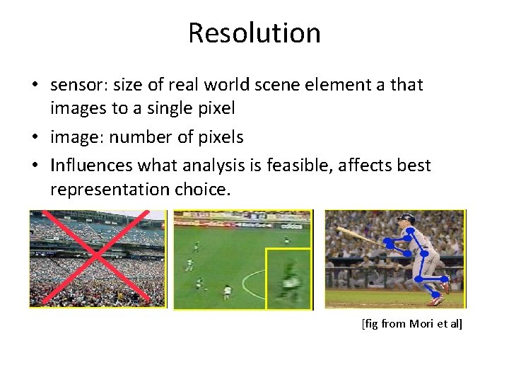
Resolution • sensor: size of real world scene element a that images to a single pixel • image: number of pixels • Influences what analysis is feasible, affects best representation choice. [fig from Mori et al]

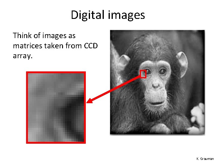
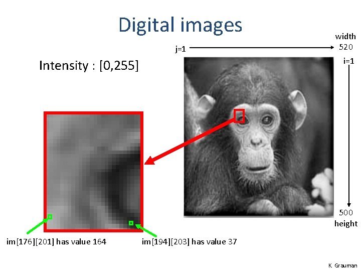
Digital images Think of images as matrices taken from CCD array. K. Grauman

Digital images j=1 width 520 i=1 Intensity : [0, 255] 500 height im[176][201] has value 164 im[194][203] has value 37 K. Grauman

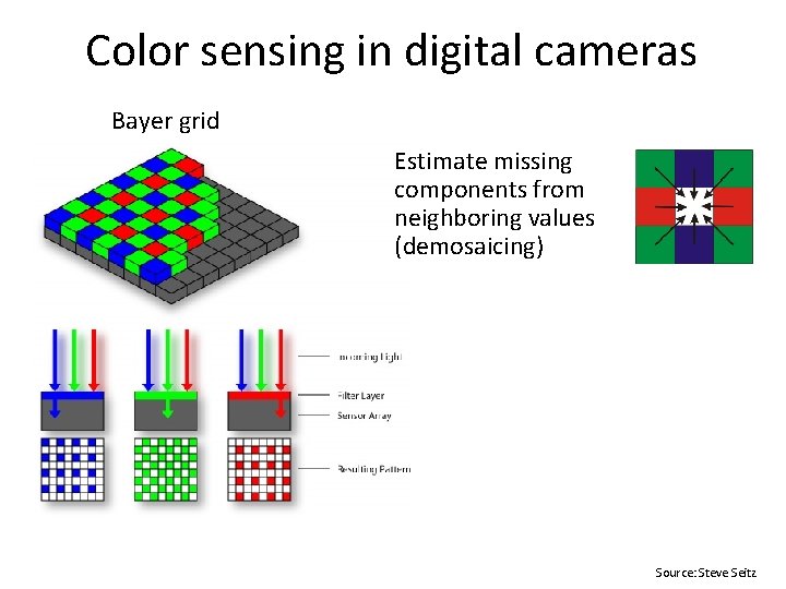
Color sensing in digital cameras Bayer grid Estimate missing components from neighboring values (demosaicing) Source: Steve Seitz

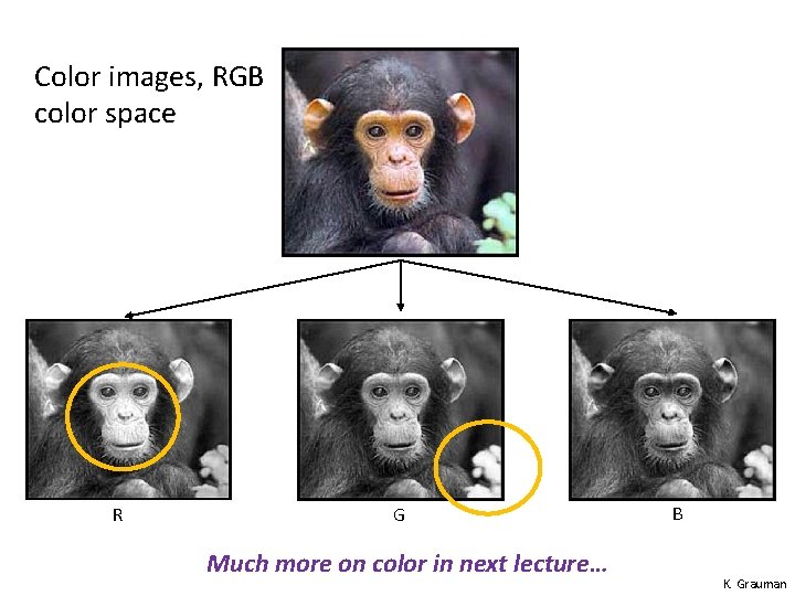
Color images, RGB color space R G Much more on color in next lecture… B K. Grauman

Physical parameters of image formation • Geometric – Type of projection – Camera pose • Optical – Sensor’s lens type – focal length, field of view, aperture • Photometric – Type, direction, intensity of light reaching sensor – Surfaces’ reflectance properties • Sensor – sampling, etc.

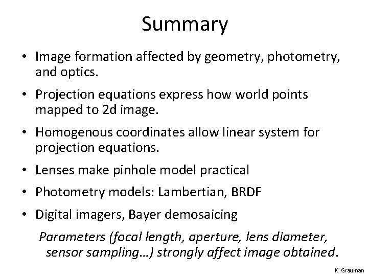
Summary • Image formation affected by geometry, photometry, and optics. • Projection equations express how world points mapped to 2 d image. • Homogenous coordinates allow linear system for projection equations. • Lenses make pinhole model practical • Photometry models: Lambertian, BRDF • Digital imagers, Bayer demosaicing Parameters (focal length, aperture, lens diameter, sensor sampling…) strongly affect image obtained. K. Grauman

Slide Credits • • • Bill Freeman Steve Seitz Kristen Grauman Forsyth and Ponce Rick Szeliski and others, as marked…

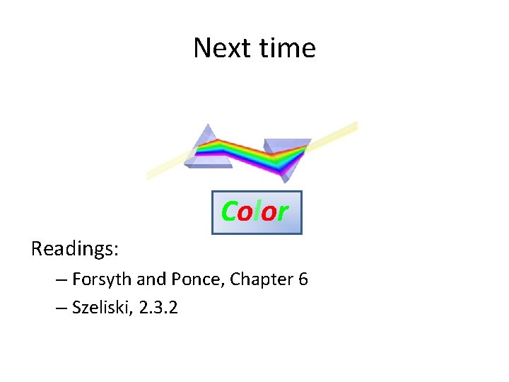
Next time ` Color Readings: – Forsyth and Ponce, Chapter 6 – Szeliski, 2. 3. 2