Business Statistics Chapter 2 Charts Graphs by Ken

Business Statistics Chapter 2 Charts & Graphs by Ken Black SP

Learning Objectives • Recognize the difference between grouped and ungrouped data • Construct a frequency distribution • Construct a histogram, a frequency polygon, an ogive, a pie chart, a stem and leaf plot, a Pareto chart, and a scatter plot SP

Ungrouped Versus Grouped Data • Ungrouped data • have not been summarized in any way • are also called raw data • Grouped data • have been organized into a frequency distribution SP

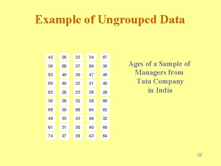
Example of Ungrouped Data 42 26 32 34 57 30 58 37 50 30 53 40 30 47 49 50 40 32 31 40 52 28 23 35 25 30 36 32 26 50 55 30 58 64 52 49 33 43 46 32 61 31 30 40 60 74 37 29 43 54 Ages of a Sample of Managers from Tata Company in India SP

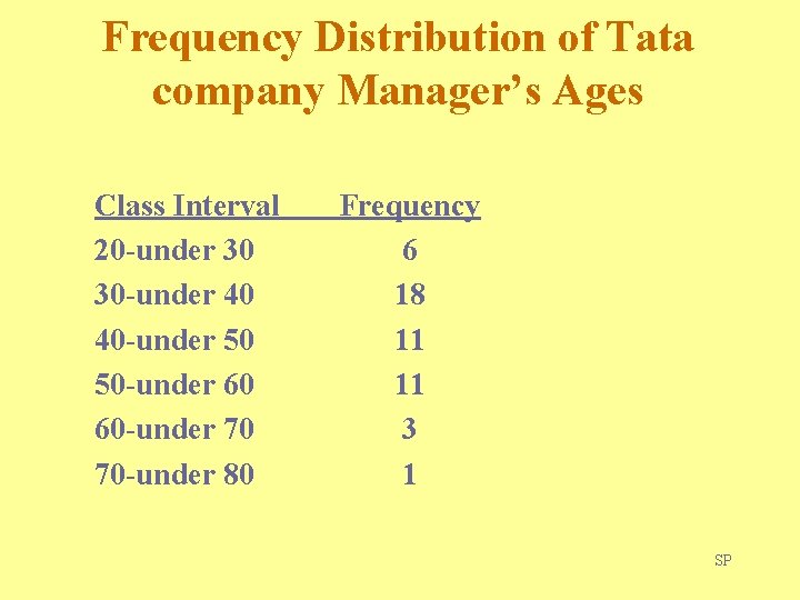
Frequency Distribution of Tata company Manager’s Ages Class Interval 20 -under 30 30 -under 40 40 -under 50 50 -under 60 60 -under 70 70 -under 80 Frequency 6 18 11 11 3 1 SP

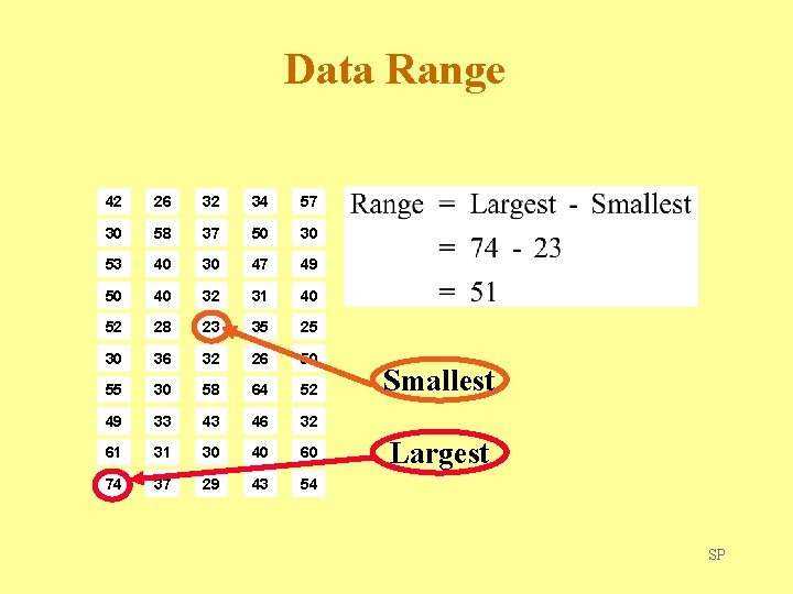
Data Range 42 26 32 34 57 30 58 37 50 30 53 40 30 47 49 50 40 32 31 40 52 28 23 35 25 30 36 32 26 50 55 30 58 64 52 49 33 43 46 32 61 31 30 40 60 74 37 29 43 54 Smallest Largest SP

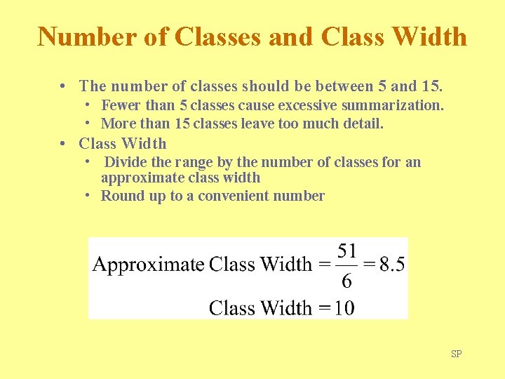
Number of Classes and Class Width • The number of classes should be between 5 and 15. • Fewer than 5 classes cause excessive summarization. • More than 15 classes leave too much detail. • Class Width • Divide the range by the number of classes for an approximate class width • Round up to a convenient number SP

Class Midpoint SP

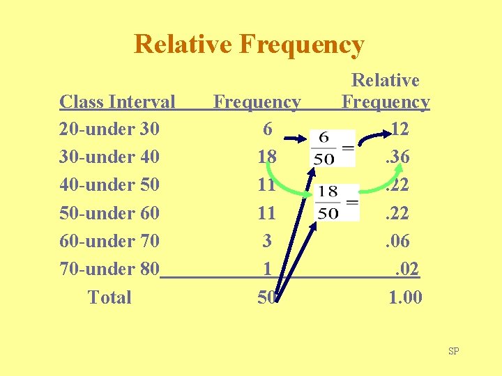
Relative Frequency Class Interval 20 -under 30 30 -under 40 40 -under 50 50 -under 60 60 -under 70 70 -under 80 Total Frequency 6 18 11 11 3 1 50 Relative Frequency. 12. 36. 22. 06. 02 1. 00 SP

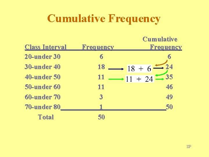
Cumulative Frequency Class Interval 20 -under 30 30 -under 40 40 -under 50 50 -under 60 60 -under 70 70 -under 80 Total Frequency 6 18 11 11 3 1 50 Cumulative Frequency 6 24 35 46 49 50 SP

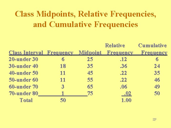
Class Midpoints, Relative Frequencies, and Cumulative Frequencies Relative Cumulative Class Interval Frequency Midpoint Frequency 20 -under 30 6 25. 12 6 30 -under 40 18 35. 36 24 40 -under 50 11 45. 22 35 50 -under 60 11 55. 22 46 60 -under 70 3 65. 06 49 70 -under 80 1 75. 02 50 Total 50 1. 00 SP

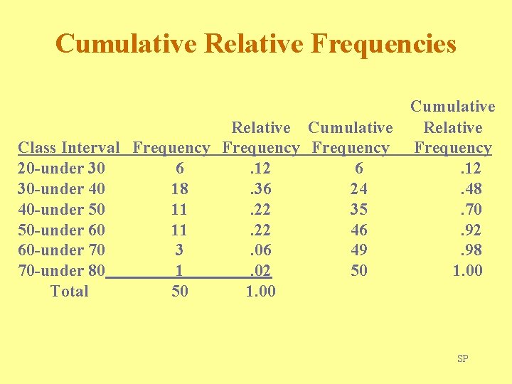
Cumulative Relative Frequencies Relative Cumulative Class Interval Frequency 20 -under 30 6. 12 6 30 -under 40 18. 36 24 40 -under 50 11. 22 35 50 -under 60 11. 22 46 60 -under 70 3. 06 49 70 -under 80 1. 02 50 Total 50 1. 00 Cumulative Relative Frequency. 12. 48. 70. 92. 98 1. 00 SP

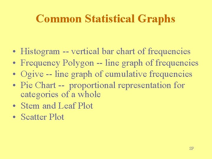
Common Statistical Graphs • • Histogram -- vertical bar chart of frequencies Frequency Polygon -- line graph of frequencies Ogive -- line graph of cumulative frequencies Pie Chart -- proportional representation for categories of a whole • Stem and Leaf Plot • Scatter Plot SP

Histogram Class Interval Frequency 20 -under 30 6 30 -under 40 18 40 -under 50 11 50 -under 60 11 60 -under 70 3 70 -under 80 1 SP

Histogram Construction Class Interval Frequency 20 -under 30 6 30 -under 40 18 40 -under 50 11 50 -under 60 11 60 -under 70 3 70 -under 80 1 SP

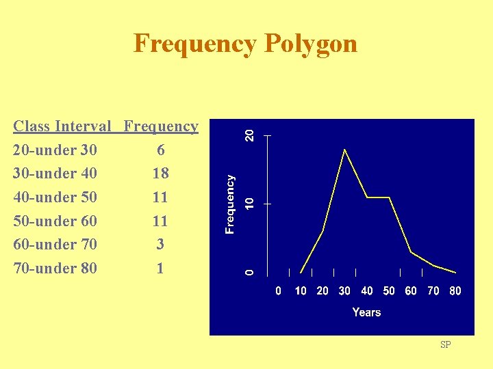
Frequency Polygon Class Interval Frequency 20 -under 30 6 30 -under 40 18 40 -under 50 11 50 -under 60 11 60 -under 70 3 70 -under 80 1 SP

Ogive Class Interval 20 -under 30 30 -under 40 40 -under 50 50 -under 60 60 -under 70 70 -under 80 Cumulative Frequency 6 24 35 46 49 50 SP

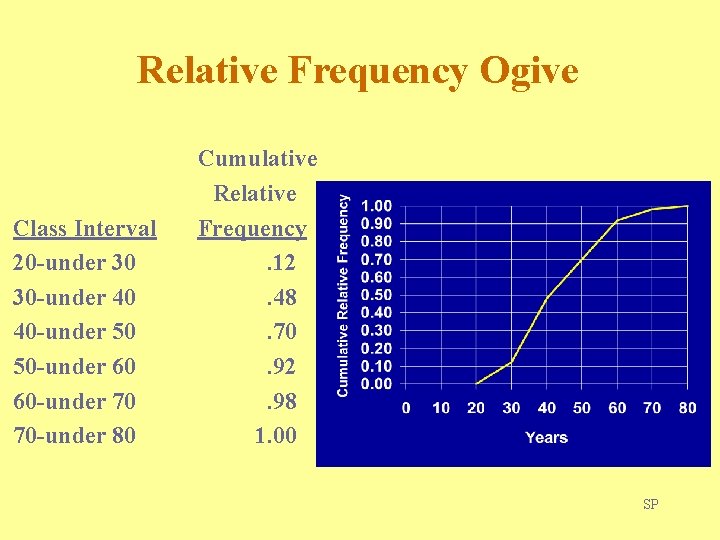
Relative Frequency Ogive Class Interval 20 -under 30 30 -under 40 40 -under 50 50 -under 60 60 -under 70 70 -under 80 Cumulative Relative Frequency. 12. 48. 70. 92. 98 1. 00 SP

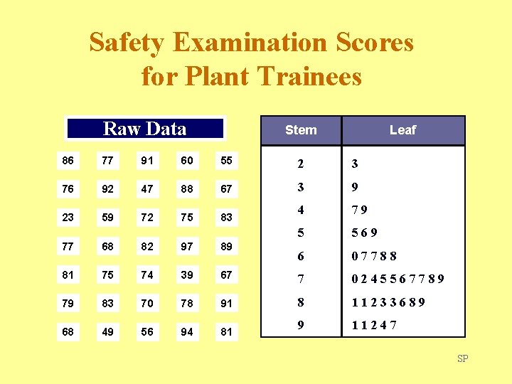
Safety Examination Scores for Plant Trainees Raw Data Stem Leaf 86 77 91 60 55 2 3 76 92 47 88 67 3 9 23 59 72 75 83 4 79 5 569 6 07788 77 68 82 97 89 81 75 74 39 67 7 0245567789 79 83 70 78 91 8 11233689 68 49 56 94 81 9 11247 SP

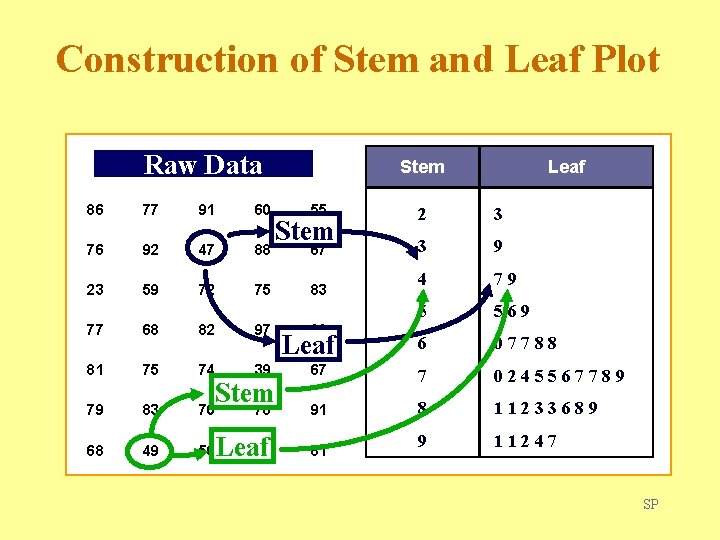
Construction of Stem and Leaf Plot Raw Data 86 77 91 60 76 92 47 88 23 59 72 75 77 68 82 97 81 75 74 39 79 83 70 68 49 56 Stem 94 Leaf 55 2 3 67 3 9 4 79 5 569 6 07788 67 7 0245567789 91 8 11233689 9 11247 Stem 78 Leaf 83 89 Leaf 81 SP

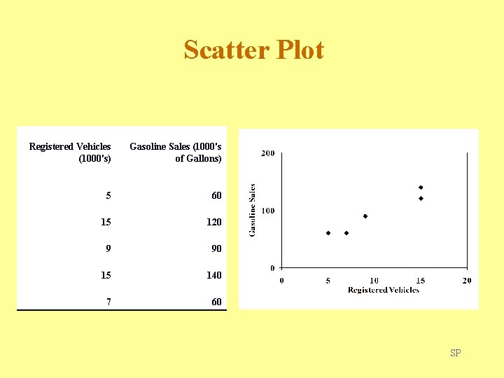
Scatter Plot Registered Vehicles (1000's) Gasoline Sales (1000's of Gallons) 5 60 15 120 9 90 15 140 7 60 SP

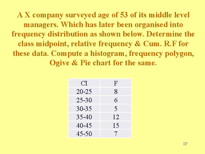
A X company surveyed age of 53 of its middle level managers. Which has later been organised into frequency distribution as shown below. Determine the class midpoint, relative frequency & Cum. R. F for these data. Compute a histogram, frequency polygon, Ogive & Pie chart for the same. CI 20 -25 25 -30 30 -35 35 -40 40 -45 45 -50 F 8 6 5 12 15 7 SP

Thank U SP