
Business Statistics 4 e by Ken Black Chapter
Business Statistics, 4 e by Ken Black Chapter 17 Nonparametric Statistics Business Statistics, 4 e, by Ken Black. © 2003 John Wiley & Sons. 1
Learning Objectives • Recognize the advantages and disadvantages of nonparametric statistics. • Understand how to use the runs test to test for randomness. • Know when and how to use the Mann-Whitney U test, the Wilcoxon matched-pairs signed rank test, the Kruskal-Wallis test, and the Friedman test. • Learn when and how to measure correlation using Spearman’s rank correlation measurement. Business Statistics, 4 e, by Ken Black. © 2003 John Wiley & Sons. 2
Parametric vs Nonparametric Statistics • Parametric Statistics are statistical techniques based on assumptions about the population from which the sample data are collected. – Assumption that data being analyzed are randomly selected from a normally distributed population. – Requires quantitative measurement that yield interval or ratio level data. • Nonparametric Statistics are based on fewer assumptions about the population and the parameters. – Sometimes called “distribution-free” statistics. – A variety of nonparametric statistics are available for use with nominal or ordinal data. Business Statistics, 4 e, by Ken Black. © 2003 John Wiley & Sons. 3
Advantages of Nonparametric Techniques • Sometimes there is no parametric alternative to the use of nonparametric statistics. • Certain nonparametric test can be used to analyze nominal data. • Certain nonparametric test can be used to analyze ordinal data. • The computations on nonparametric statistics are usually less complicated than those for parametric statistics, particularly for small samples. • Probability statements obtained from most nonparametric tests are exact probabilities. Business Statistics, 4 e, by Ken Black. © 2003 John Wiley & Sons. 4
Disadvantages of Nonparametric Statistics • Nonparametric tests can be wasteful of data if parametric tests are available for use with the data. • Nonparametric tests are usually not as widely available and well know as parametric tests. • For large samples, the calculations for many nonparametric statistics can be tedious. Business Statistics, 4 e, by Ken Black. © 2003 John Wiley & Sons. 5
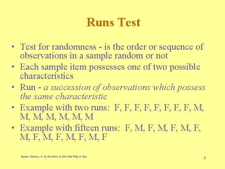
Runs Test • Test for randomness - is the order or sequence of observations in a sample random or not • Each sample item possesses one of two possible characteristics • Run - a succession of observations which possess the same characteristic • Example with two runs: F, F, M, M, M, M • Example with fifteen runs: F, M, F, M, F Business Statistics, 4 e, by Ken Black. © 2003 John Wiley & Sons. 6
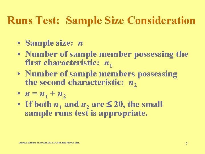
Runs Test: Sample Size Consideration • Sample size: n • Number of sample member possessing the first characteristic: n 1 • Number of sample members possessing the second characteristic: n 2 • n = n 1 + n 2 • If both n 1 and n 2 are 20, the small sample runs test is appropriate. Business Statistics, 4 e, by Ken Black. © 2003 John Wiley & Sons. 7

Runs Test: Small Sample Example H 0: The observations in the sample are randomly generated. Ha: The observations in the sample are not randomly generated. =. 05 n 1 = 18 n 2 = 8 If 7 R 17, do not reject H 0 Otherwise, reject H 0. 1 2 3 4 5 6 7 8 9 10 11 12 D CCCCC D CCC DDD CCC R = 12 Since 7 R = 12 17, do not reject H 0 Business Statistics, 4 e, by Ken Black. © 2003 John Wiley & Sons. 8
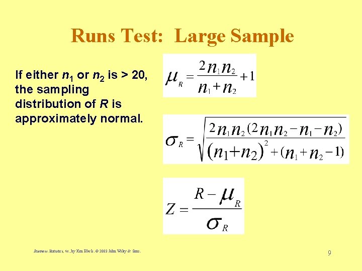
Runs Test: Large Sample If either n 1 or n 2 is > 20, the sampling distribution of R is approximately normal. Business Statistics, 4 e, by Ken Black. © 2003 John Wiley & Sons. 9
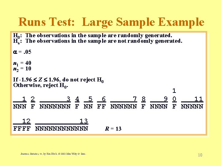
Runs Test: Large Sample Example H 0: The observations in the sample are randomly generated. Ha: The observations in the sample are not randomly generated. =. 05 n 1 = 40 n 2 = 10 If -1. 96 Z 1. 96, do not reject H 0 Otherwise, reject H 0. 1 1 2 3 4 5 6 7 8 9 0 11 NNN F NNNNNNN FF NNNNNN F NNNNN 12 13 FFFF NNNNNN Business Statistics, 4 e, by Ken Black. © 2003 John Wiley & Sons. R = 13 10
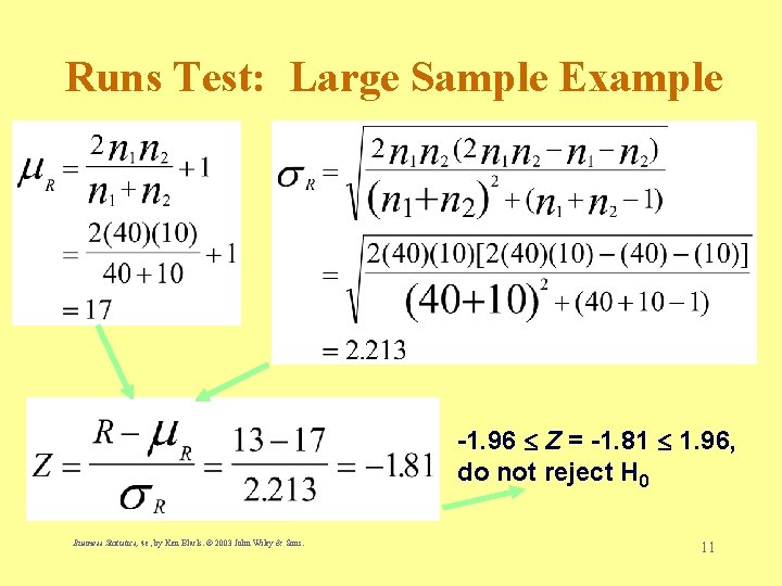
Runs Test: Large Sample Example -1. 96 Z = -1. 81 1. 96, do not reject H 0 Business Statistics, 4 e, by Ken Black. © 2003 John Wiley & Sons. 11
Mann-Whitney U Test • Nonparametric counterpart of the t test for independent samples • Does not require normally distributed populations • May be applied to ordinal data • Assumptions – Independent Samples – At Least Ordinal Data Business Statistics, 4 e, by Ken Black. © 2003 John Wiley & Sons. 12
Mann-Whitney U Test: Sample Size Consideration • Size of sample one: n 1 • Size of sample two: n 2 • If both n 1 and n 2 are 10, the small sample procedure is appropriate. • If either n 1 or n 2 is greater than 10, the large sample procedure is appropriate. Business Statistics, 4 e, by Ken Black. © 2003 John Wiley & Sons. 13
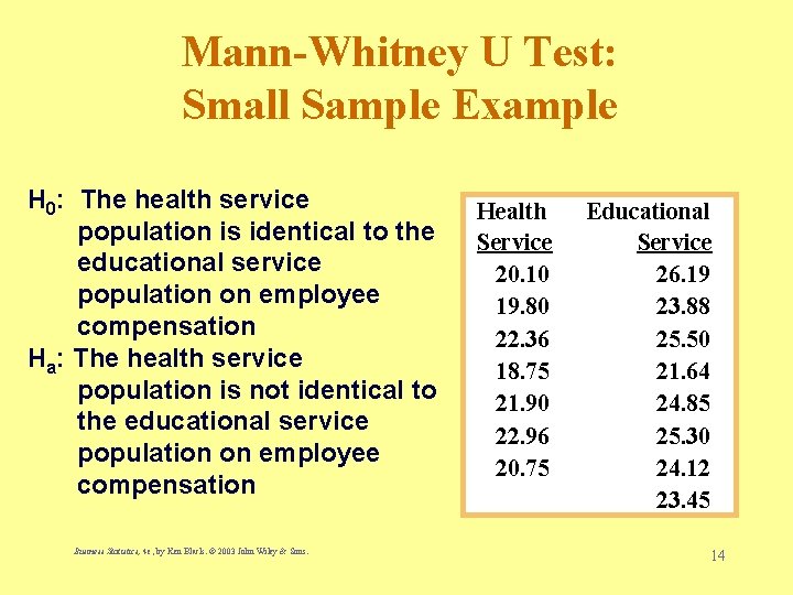
Mann-Whitney U Test: Small Sample Example H 0: The health service population is identical to the educational service population on employee compensation Ha: The health service population is not identical to the educational service population on employee compensation Business Statistics, 4 e, by Ken Black. © 2003 John Wiley & Sons. Health Service 20. 10 19. 80 22. 36 18. 75 21. 90 22. 96 20. 75 Educational Service 26. 19 23. 88 25. 50 21. 64 24. 85 25. 30 24. 12 23. 45 14
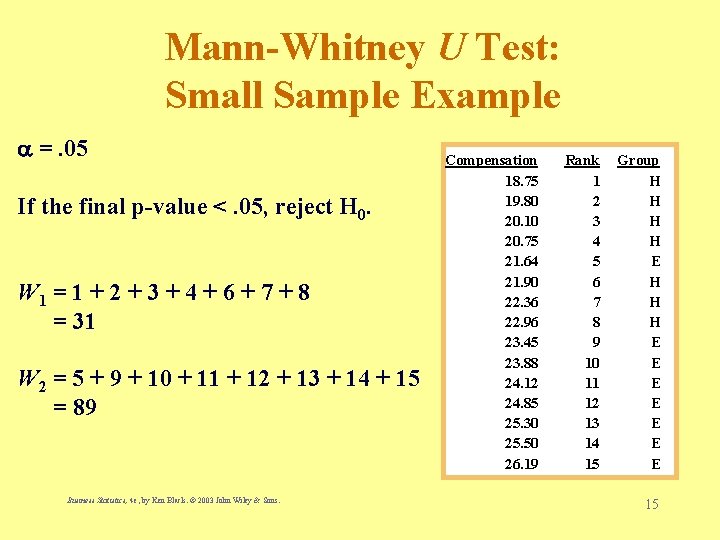
Mann-Whitney U Test: Small Sample Example =. 05 If the final p-value <. 05, reject H 0. W 1 = 1 + 2 + 3 + 4 + 6 + 7 + 8 = 31 W 2 = 5 + 9 + 10 + 11 + 12 + 13 + 14 + 15 = 89 Business Statistics, 4 e, by Ken Black. © 2003 John Wiley & Sons. Compensation 18. 75 19. 80 20. 10 20. 75 21. 64 21. 90 22. 36 22. 96 23. 45 23. 88 24. 12 24. 85 25. 30 25. 50 26. 19 Rank 1 2 3 4 5 6 7 8 9 10 11 12 13 14 15 Group H H E H H H E E E E 15
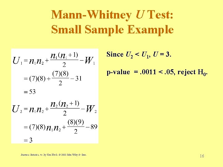
Mann-Whitney U Test: Small Sample Example Since U 2 < U 1, U = 3. p-value =. 0011 <. 05, reject H 0. Business Statistics, 4 e, by Ken Black. © 2003 John Wiley & Sons. 16
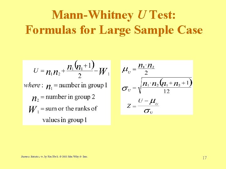
Mann-Whitney U Test: Formulas for Large Sample Case Business Statistics, 4 e, by Ken Black. © 2003 John Wiley & Sons. 17
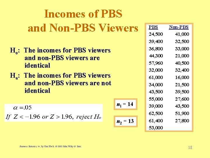
Incomes of PBS and Non-PBS Viewers Ho: The incomes for PBS viewers and non-PBS viewers are identical Ha: The incomes for PBS viewers and non-PBS viewers are not identical n 1 = 14 n 2 = 13 Business Statistics, 4 e, by Ken Black. © 2003 John Wiley & Sons. PBS 24, 500 39, 400 36, 800 44, 300 57, 960 32, 000 61, 000 34, 000 43, 500 55, 000 39, 000 62, 500 61, 400 53, 000 Non-PBS 41, 000 32, 500 33, 000 21, 000 40, 500 32, 400 16, 000 21, 500 39, 500 27, 600 43, 500 51, 900 27, 800 18
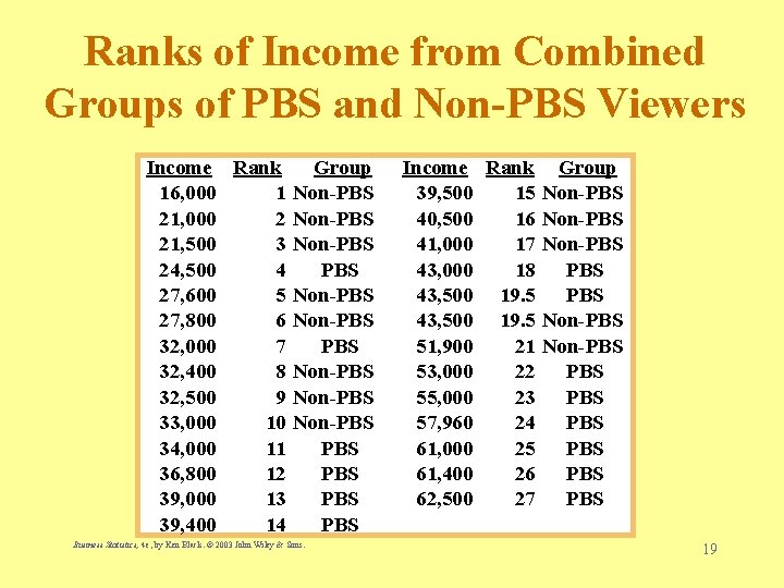
Ranks of Income from Combined Groups of PBS and Non-PBS Viewers Income Rank Group 16, 000 1 Non-PBS 21, 000 2 Non-PBS 21, 500 3 Non-PBS 24, 500 4 PBS 27, 600 5 Non-PBS 27, 800 6 Non-PBS 32, 000 7 PBS 32, 400 8 Non-PBS 32, 500 9 Non-PBS 33, 000 10 Non-PBS 34, 000 11 PBS 36, 800 12 PBS 39, 000 13 PBS 39, 400 14 PBS Business Statistics, 4 e, by Ken Black. © 2003 John Wiley & Sons. Income Rank Group 39, 500 15 Non-PBS 40, 500 16 Non-PBS 41, 000 17 Non-PBS 43, 000 18 PBS 43, 500 19. 5 Non-PBS 51, 900 21 Non-PBS 53, 000 22 PBS 55, 000 23 PBS 57, 960 24 PBS 61, 000 25 PBS 61, 400 26 PBS 62, 500 27 PBS 19
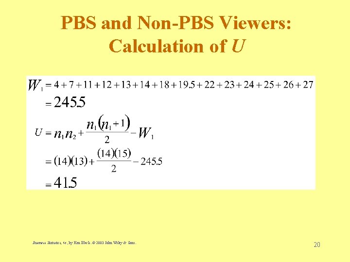
PBS and Non-PBS Viewers: Calculation of U Business Statistics, 4 e, by Ken Black. © 2003 John Wiley & Sons. 20
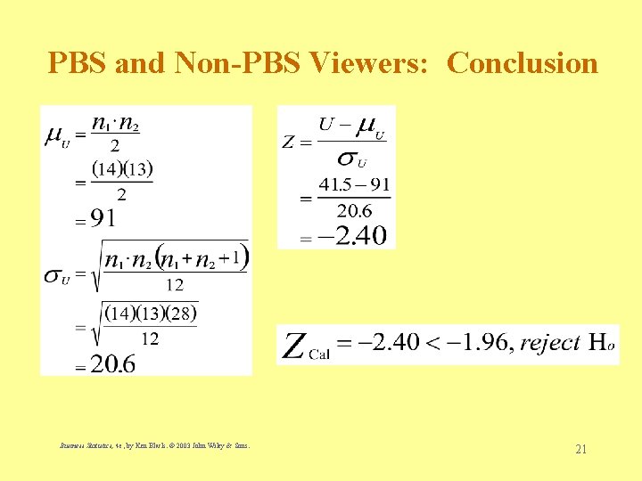
PBS and Non-PBS Viewers: Conclusion Business Statistics, 4 e, by Ken Black. © 2003 John Wiley & Sons. 21
Wilcoxon Matched-Pairs Signed Rank Test • A nonparametric alternative to the t test for related samples • Before and After studies • Studies in which measures are taken on the same person or object under different conditions • Studies or twins or other relatives Business Statistics, 4 e, by Ken Black. © 2003 John Wiley & Sons. 22
Wilcoxon Matched-Pairs Signed Rank Test • Differences of the scores of the two matched samples • Differences are ranked, ignoring the sign • Ranks are given the sign of the difference • Positive ranks are summed • Negative ranks are summed • T is the smaller sum of ranks Business Statistics, 4 e, by Ken Black. © 2003 John Wiley & Sons. 23
Wilcoxon Matched-Pairs Signed Rank Test: Sample Size Consideration • n is the number of matched pairs • If n > 15, T is approximately normally distributed, and a Z test is used. • If n 15, a special “small sample” procedure is followed. – The paired data are randomly selected. – The underlying distributions are symmetrical. Business Statistics, 4 e, by Ken Black. © 2003 John Wiley & Sons. 24
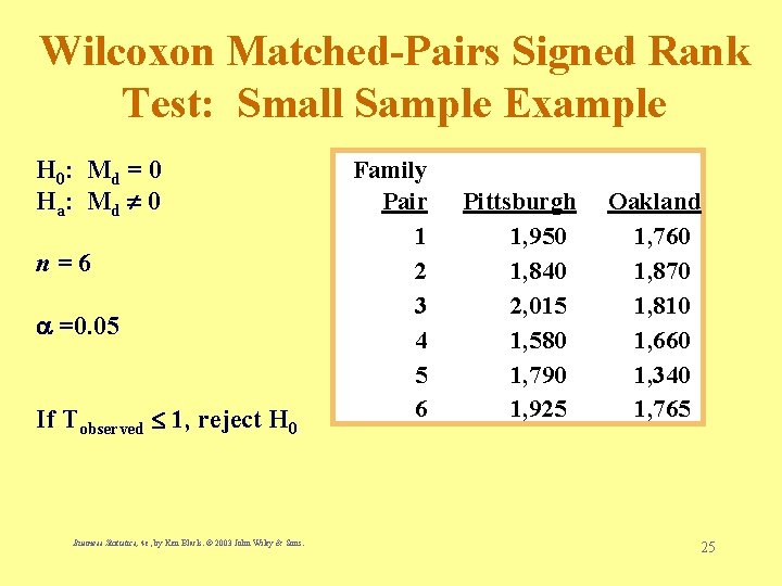
Wilcoxon Matched-Pairs Signed Rank Test: Small Sample Example H 0: M d = 0 H a: M d 0 n=6 =0. 05 If Tobserved 1, reject H 0. Business Statistics, 4 e, by Ken Black. © 2003 John Wiley & Sons. Family Pair 1 2 3 4 5 6 Pittsburgh 1, 950 1, 840 2, 015 1, 580 1, 790 1, 925 Oakland 1, 760 1, 870 1, 810 1, 660 1, 340 1, 765 25
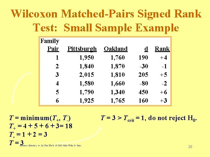
Wilcoxon Matched-Pairs Signed Rank Test: Small Sample Example Family Pair 1 2 3 4 5 6 Pittsburgh 1, 950 1, 840 2, 015 1, 580 1, 790 1, 925 T = minimum(T+, T-) T+ = 4 + 5 + 6 + 3= 18 T- = 1 + 2 = 3 T=3 Business Statistics, 4 e, by Ken Black. © 2003 John Wiley & Sons. Oakland 1, 760 1, 870 1, 810 1, 660 1, 340 1, 765 d 190 -30 205 -80 450 160 Rank +4 -1 +5 -2 +6 +3 T = 3 > Tcrit = 1, do not reject H 0. 26
Wilcoxon Matched-Pairs Signed Rank Test: Large Sample Formulas Business Statistics, 4 e, by Ken Black. © 2003 John Wiley & Sons. 27
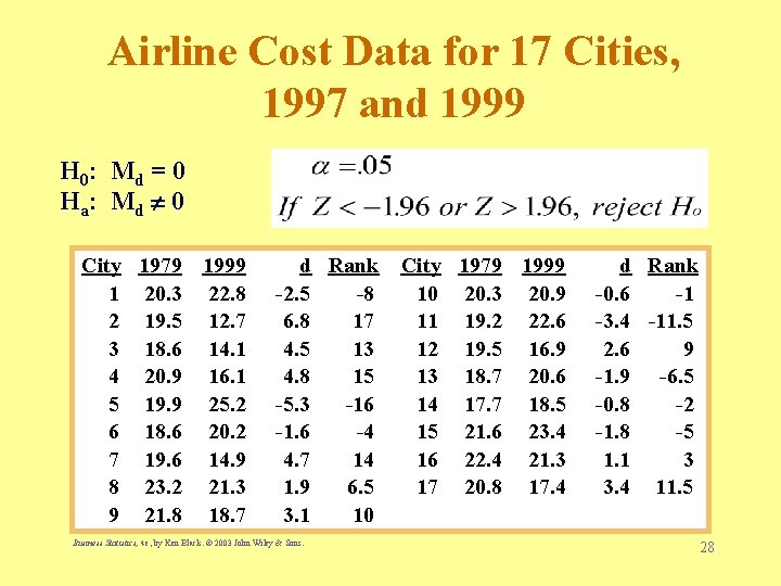
Airline Cost Data for 17 Cities, 1997 and 1999 H 0: M d = 0 H a: M d 0 City 1979 1999 1 20. 3 22. 8 2 19. 5 12. 7 3 18. 6 14. 1 4 20. 9 16. 1 5 19. 9 25. 2 6 18. 6 20. 2 7 19. 6 14. 9 8 23. 2 21. 3 9 21. 8 18. 7 d Rank -2. 5 -8 6. 8 17 4. 5 13 4. 8 15 -5. 3 -16 -1. 6 -4 4. 7 14 1. 9 6. 5 3. 1 10 Business Statistics, 4 e, by Ken Black. © 2003 John Wiley & Sons. City 1979 1999 10 20. 3 20. 9 11 19. 2 22. 6 12 19. 5 16. 9 13 18. 7 20. 6 14 17. 7 18. 5 15 21. 6 23. 4 16 22. 4 21. 3 17 20. 8 17. 4 d Rank -0. 6 -1 -3. 4 -11. 5 2. 6 9 -1. 9 -6. 5 -0. 8 -2 -1. 8 -5 1. 1 3 3. 4 11. 5 28
Airline Cost: T Calculation Business Statistics, 4 e, by Ken Black. © 2003 John Wiley & Sons. 29
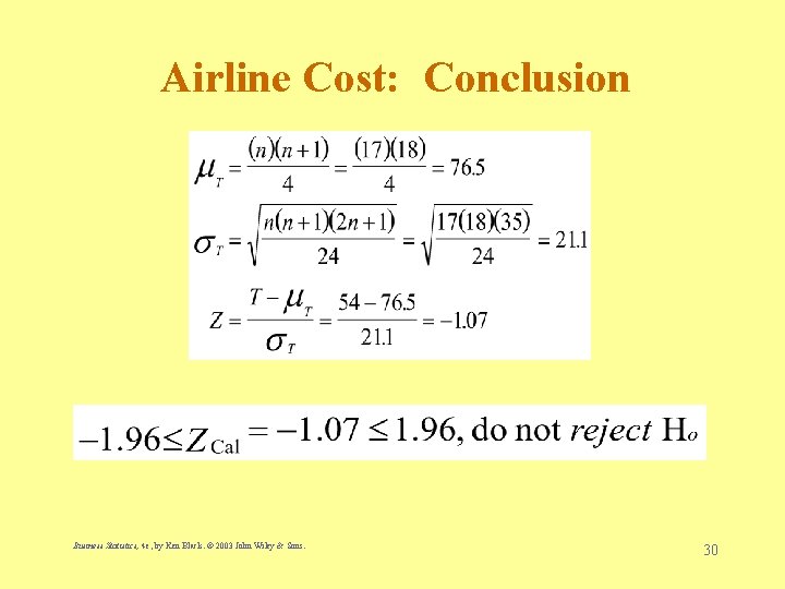
Airline Cost: Conclusion Business Statistics, 4 e, by Ken Black. © 2003 John Wiley & Sons. 30
Kruskal-Wallis Test • A nonparametric alternative to one-way analysis of variance • May used to analyze ordinal data • No assumed population shape • Assumes that the C groups are independent • Assumes random selection of individual items Business Statistics, 4 e, by Ken Black. © 2003 John Wiley & Sons. 31
Kruskal-Wallis K Statistic Business Statistics, 4 e, by Ken Black. © 2003 John Wiley & Sons. 32
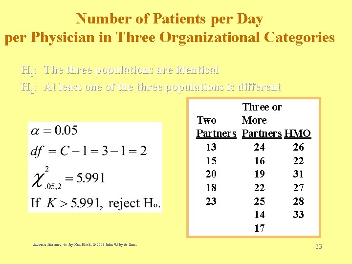
Number of Patients per Day per Physician in Three Organizational Categories Ho: The three populations are identical Ha: At least one of the three populations is different Three or Two More Partners HMO 13 24 26 15 16 22 20 19 31 18 22 27 23 25 28 14 33 17 Business Statistics, 4 e, by Ken Black. © 2003 John Wiley & Sons. 33
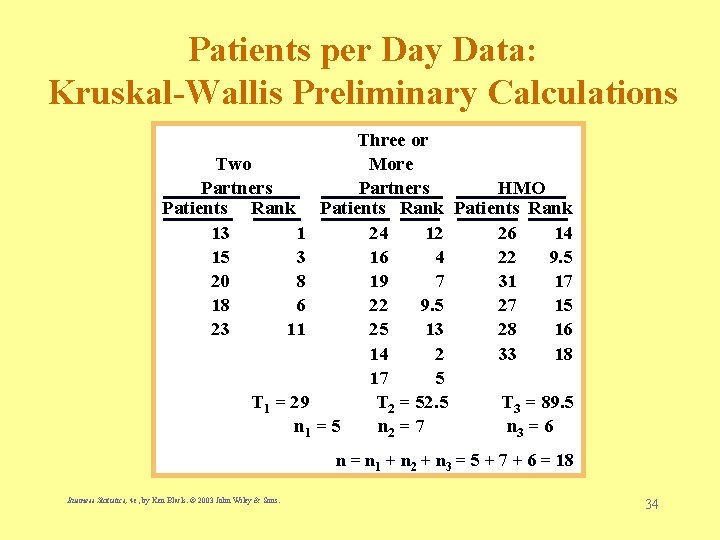
Patients per Day Data: Kruskal-Wallis Preliminary Calculations Three or Two More Partners HMO Patients Rank 13 1 24 12 26 14 15 3 16 4 22 9. 5 20 8 19 7 31 17 18 6 22 9. 5 27 15 23 11 25 13 28 16 14 2 33 18 17 5 T 1 = 29 T 2 = 52. 5 T 3 = 89. 5 n 1 = 5 n 2 = 7 n 3 = 6 n = n 1 + n 2 + n 3 = 5 + 7 + 6 = 18 Business Statistics, 4 e, by Ken Black. © 2003 John Wiley & Sons. 34
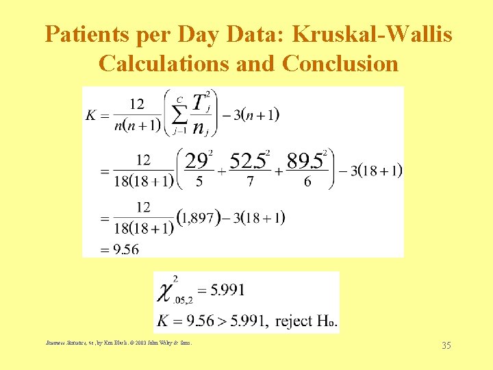
Patients per Day Data: Kruskal-Wallis Calculations and Conclusion Business Statistics, 4 e, by Ken Black. © 2003 John Wiley & Sons. 35
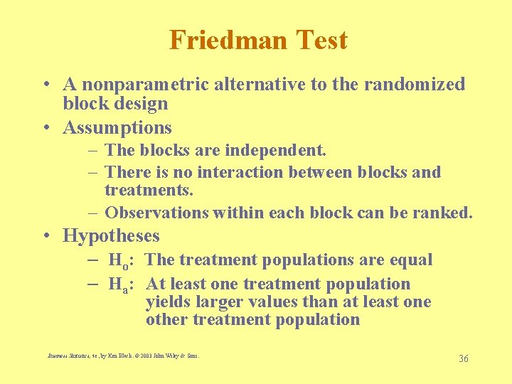
Friedman Test • A nonparametric alternative to the randomized block design • Assumptions – The blocks are independent. – There is no interaction between blocks and treatments. – Observations within each block can be ranked. • Hypotheses – Ho: The treatment populations are equal – Ha: At least one treatment population yields larger values than at least one other treatment population Business Statistics, 4 e, by Ken Black. © 2003 John Wiley & Sons. 36
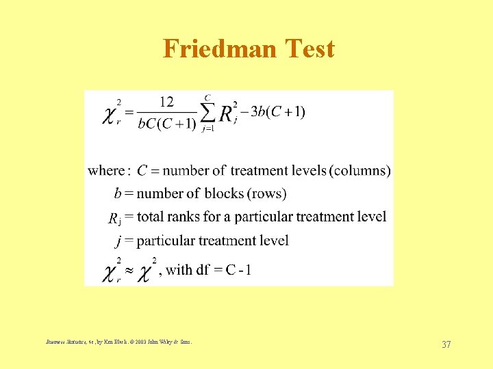
Friedman Test Business Statistics, 4 e, by Ken Black. © 2003 John Wiley & Sons. 37
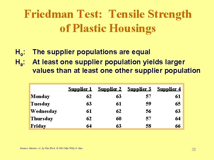
Friedman Test: Tensile Strength of Plastic Housings Ho: The supplier populations are equal Ha: At least one supplier population yields larger values than at least one other supplier population Monday Tuesday Wednesday Thursday Friday Supplier 1 62 63 61 62 64 Business Statistics, 4 e, by Ken Black. © 2003 John Wiley & Sons. Supplier 2 63 61 62 60 63 Supplier 3 57 59 56 57 58 Supplier 4 61 65 63 64 66 38
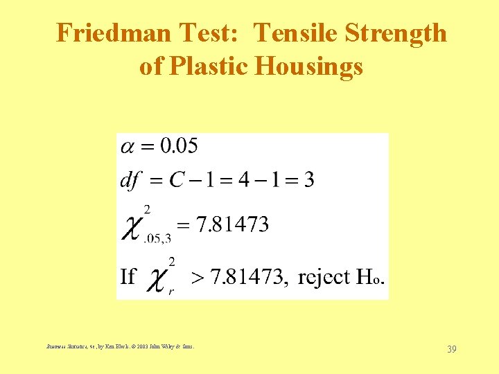
Friedman Test: Tensile Strength of Plastic Housings Business Statistics, 4 e, by Ken Black. © 2003 John Wiley & Sons. 39
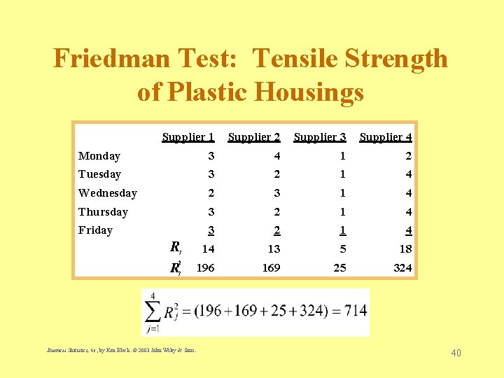
Friedman Test: Tensile Strength of Plastic Housings Supplier 1 Supplier 2 Supplier 3 Supplier 4 Monday 3 4 1 2 Tuesday 3 2 1 4 Wednesday 2 3 1 4 Thursday 3 2 1 4 Friday 3 2 1 4 14 13 5 18 196 169 25 324 R R j 2 j Business Statistics, 4 e, by Ken Black. © 2003 John Wiley & Sons. 40
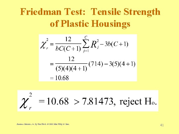
Friedman Test: Tensile Strength of Plastic Housings Business Statistics, 4 e, by Ken Black. © 2003 John Wiley & Sons. 41
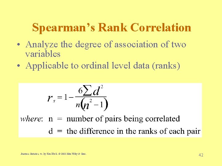
Spearman’s Rank Correlation • Analyze the degree of association of two variables • Applicable to ordinal level data (ranks) Business Statistics, 4 e, by Ken Black. © 2003 John Wiley & Sons. 42
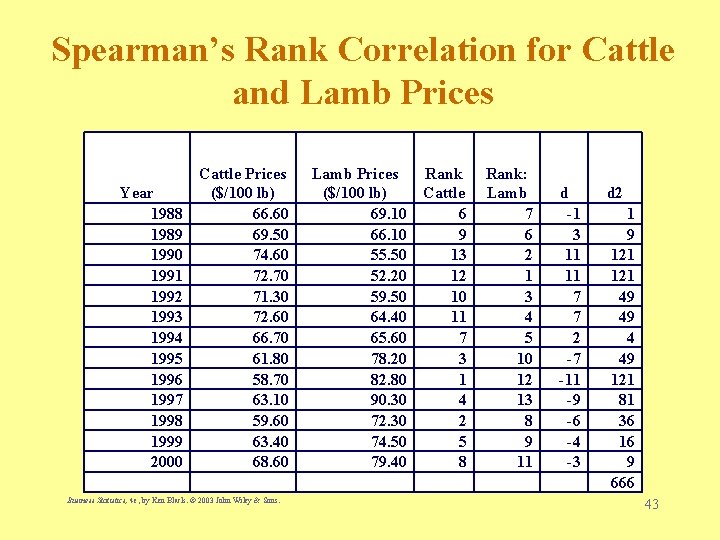
Spearman’s Rank Correlation for Cattle and Lamb Prices Year 1988 1989 1990 1991 1992 1993 1994 1995 1996 1997 1998 1999 2000 Cattle Prices ($/100 lb) 66. 60 69. 50 74. 60 72. 70 71. 30 72. 60 66. 70 61. 80 58. 70 63. 10 59. 60 63. 40 68. 60 Business Statistics, 4 e, by Ken Black. © 2003 John Wiley & Sons. Lamb Prices ($/100 lb) 69. 10 66. 10 55. 50 52. 20 59. 50 64. 40 65. 60 78. 20 82. 80 90. 30 72. 30 74. 50 79. 40 Rank Cattle 6 9 13 12 10 11 7 3 1 4 2 5 8 Rank: Lamb 7 6 2 1 3 4 5 10 12 13 8 9 11 d -1 3 11 11 7 7 2 -7 -11 -9 -6 -4 -3 d 2 1 9 121 49 49 4 49 121 81 36 16 9 666 43
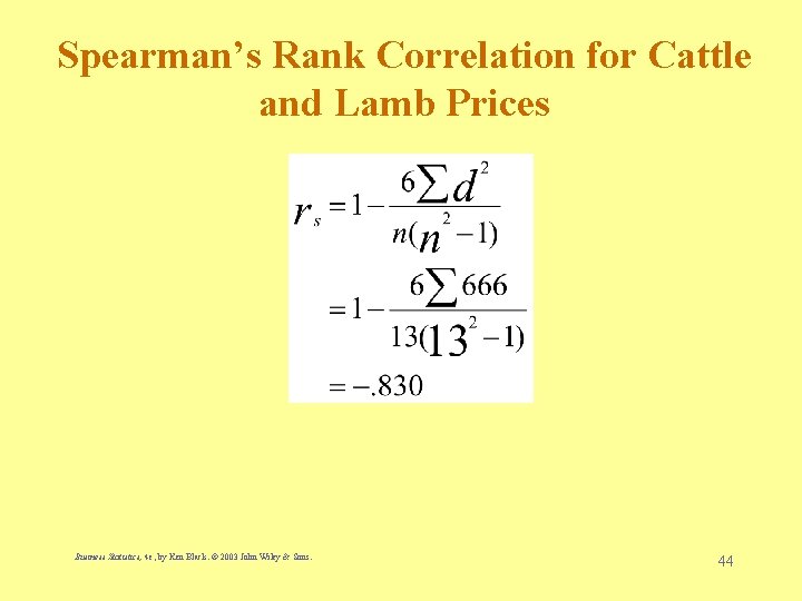
Spearman’s Rank Correlation for Cattle and Lamb Prices Business Statistics, 4 e, by Ken Black. © 2003 John Wiley & Sons. 44
- Slides: 44