BUSINESS MATHEMATICS STATISTICS LECTURE 26 Review Lecture 25

BUSINESS MATHEMATICS & STATISTICS

LECTURE 26 Review Lecture 25 Statistical Representation Measures of Dispersion and Skewness Part 1

GRAPHING NUMERICAL DATA: THE FREQUENCY POLYGON Data in ordered array 12, 13, 17, 21, 24, 26, 27, 30, 32, 35, 37, 38, 41, 43, 44, 46, 53, 58 Class Midpoints

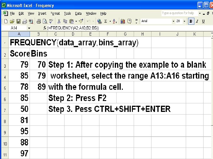
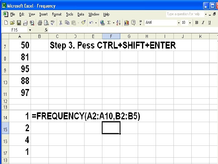
TABULATING NUMERICAL DATA: CUMULATIVE FREQUENCY Data in ordered array 12, 13, 17, 21, 24, 26, 27, 30, 32, 35, 37, 38, 41, 43, 44, 46, 53, 58 Class 10 but under 20 20 but under 30 30 but under 40 40 but under 50 50 but under 60 Cumulative Frequency 3 9 14 18 20 Cumulative % Frequency 15 45 70 90 100

GRAPHING NUMERICAL DATA: THE OGIVE (CUMULATIVE % POLYGON) Data in ordered array 12, 13, 17, 21, 24, 26, 27, 30, 32, 35, 37, 38, 41, 43, 44, 46, 53, 58 Class Boundaries (Not Midpoints)

TABULATING AND GRAPHING CATEGORICAL DATA: UNIVARIATE DATA Categorical Data Tabulating Data The Summary Table Graphing Data Pie Charts Bar Charts Pareto Diagram

SUMMARY TABLE (FOR AN INVESTOR’S PORTFOLIO) Investment Category Amount Percentage (in thousands Rs. ) Stocks Bonds CD Savings Total 46. 5 32. 0 15. 5 16 110 Variables are Categorical 42. 27 29. 09 14. 55 100

GRAPHING CATEGORICAL DATA: UNIVARIATE DATA Categorical Data Graphing Data Tabulating Data The Summary Table Pie Charts Bar Charts Pareto. Diagram

BAR CHART (FOR AN INVESTOR’S PORTFOLIO)

PIE CHART (FOR AN INVESTOR’S PORTFOLIO) Amount Invested in Rs. Savings 15% Stocks 42% CD 14% Bonds 29% Percentages are rounded to the nearest percent.

PARETO DIAGRAM Axis for bar chart shows % invested in each category Axis for line graph shows cumulative % invested

TABULATING AND GRAPHING BIVARIATE CATEGORICAL DATA Contingency Tables Side by Side Charts

TABULATING CATEGORICAL DATA: BIVARIATE DATA Contingency Table Investment Category Investment in Thousands of Rupees Investor A Investor B Investor C Stocks 129 Bonds CD Savings 46. 5 55 27. 5 32 15. 5 16 44 20 28 19 13. 5 7 Total 110 147 67 Total 95 49 51 324

GRAPHING CATEGORICAL DATA: BIVARIATE DATA Side by Side Chart

GEOMETRIC MEAN Syntax G=(x 1. x 2. x 3. . . xn)^1/n Example Find GM of 130, 140, 160 GM = (130*140*160)^1/3 = 142. 8

MARMONIC MEAN Syntax HM=n/(1/x 1+1/x 2+. . . 1/xn) =n/Sum(1/xi) Example Find HM of 10, 8, 6 HM = 3/(1/10+1/8+ 1/6) = 7. 66

BUSINESS MATHEMATICS & STATISTICS

QUARTILES Quartiles divide data into 4 equal parts Syntax 1 st Quartile Q 1=(n+1)/4 2 nd Quartile Q 2= 2(n+1)/4 3 rd Quartile Q 3= 3(n+1)/4 Grouped data Qi= ith Quartile = l + h/f[Sum f/4*i – cf) l = lower boundary h = width of CI cf = cumulative frequency

DECILES Deciles divide data into 10 equal parts Syntax 1 st Decile D 1=(n+1)/10 2 nd Decile D 2= 2(n+1)/10 9 th Deciled D 9= 9(n+1)/10 Grouped data Qi = ith Decile (i=1, 2, . 9) = l + h/f[Sum f/10*i – cf) l = lower boundary h = width of CI cf = cumulative frequency

PERCENTILES Percentiles divide data into 100 equal parts Syntax 1 st Percentile P 1=(n+1)/100 2 nd Decile D 2= 2(n+1)/100 99 th Deciled D 9= 99(n+1)/100 Grouped data Qi = ith Decile(i=1, 2, . 9) = l + h/f[Sum f/100*i – cf) l = lower boundary h = width of CI cf = cumulative frequency

EMPIRICAL RELATIONSHIPS Symmetrical Distribution mean = median = mode Positively Skewed Distribution (Tilted to left) mean > median > mode Negatively Skewed Distribution mode > median > mean (Tilted to right)

EMPIRICAL RELATIONSHIPS Moderately Skewed and Unimodal Distribution Mean – Mode = 3(Mean – Median) Example mode = 15, mean = 18, median = ? Median = 1/3[mode + 2 mean] = 1/3[15 + 2(18)] = [15+36]/3 = 51/3 = 17

MODIFIED MEANS TRIMMED MEAN Remove all observations below 1 st quartile and above 3 rd Quartile Winsorized MEAN Replace each observation below first quartile with value of first quartile Replace each observation above third quartile with value of 3 rd quartile

TRIMMED AND WINSORIZED MEAN Example Find trimmed and winsorized mean. 9. 1, 9. 2, 9. 3, 9. 2 Array the data 9. 1, 9. 2, 9. 3, 9. 9 Q 1 = (6+1)/4=1. 75 (2 nd value) = 9. 2 Q 3 = 3(6+1)/4= 5. 25 (6 th value) = 9. 3 TM= (9. 2+9. 3)/5 = 9. 22 WM = (9. 2+9. 3+9. 3)/7

DISPERSION OF DATA Definition The degree to which numerical data tend to spread about an average is called the dispersion of data TYPES OF MEASURES OF DISPERSION Absolute measures Relative measures (coefficients)

DISPERSION OF DATA TYPES OF ABSOLUTE MEASURES 1. Range 2. Quartile Deviation 3. Mean Deviation 4. Standard Deviation or Variance TYPES OF RELATIVE MEASURES 1. Coefficient of Range 2. Coefficient of Quartile Deviation 3. Coefficient of Mean Deviation 4. Coefficient of Variation

BUSINESS MATHEMATICS & STATISTICS