BUS221 Quantitative Methods LECTURE 1 Learning Outcome Knowledge

BUS-221 Quantitative Methods LECTURE 1

Learning Outcome Knowledge Describe the use and theory of indices, especially those commonly used in business. Understand quantitative theories of use in business such as forecasting, decision making, queuing theory. Mentation Argument Communication

Topics Introduction to Quantitative Analysis Approach Mathematical Modeling Excel QM Probability Concepts Types of Probability Expected Value

Introduction WHAT IS QUANTITATIVE ANALYSIS? A technique that seeks to understand behaviour by using mathematical and statistical modeling, measurement, and research. Quantitative analysis can be applied to a wide variety of problems using mathematical tools.

Examples of Quantitative Analyses Retailers can increase revenues using historical data by using quantitative analysis to develop better sales plans. Airlines saved millions of $ by using quantitative analysis models to quickly recover from weather delays and other disruptions.

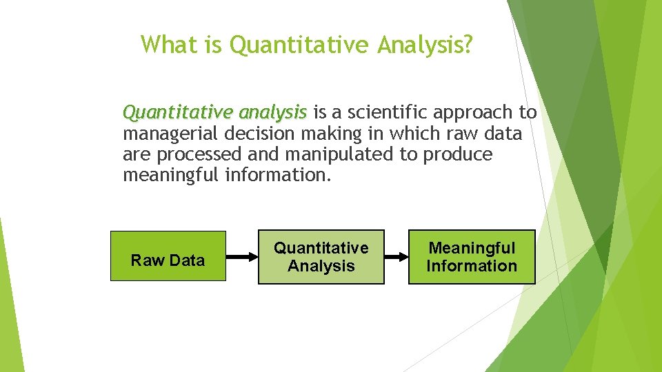
What is Quantitative Analysis? Quantitative analysis is a scientific approach to managerial decision making in which raw data are processed and manipulated to produce meaningful information. Raw Data Quantitative Analysis Meaningful Information

What is Quantitative Analysis? Quantitative factors are data that can be accurately calculated. Examples include: Different investment alternatives Diffe Interest rates Inventory levels Demand Labor cost Qualitative factors are more difficult to quantify but affect the decision process. Examples include: The weather State and federal legislation Technological breakthroughs.

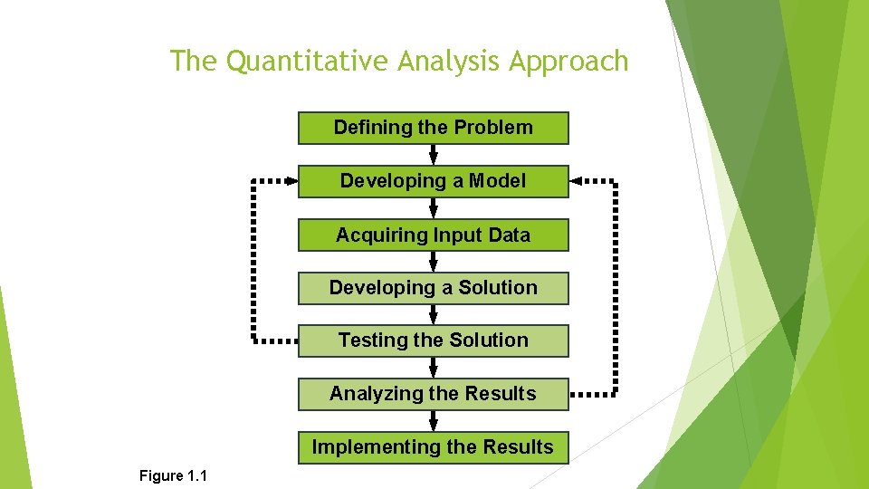
The Quantitative Analysis Approach Defining the Problem Developing a Model Acquiring Input Data Developing a Solution Testing the Solution Analyzing the Results Implementing the Results Figure 1. 1

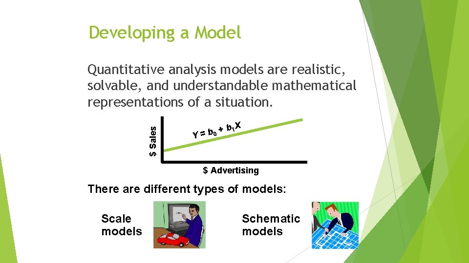
Developing a Model $ Sales Quantitative analysis models are realistic, solvable, and understandable mathematical representations of a situation. b 1 X + b 0 Y= $ Advertising There are different types of models: Scale models Schematic models

Developing a Solution The best (optimal) solution to a problem is found by manipulating the model variables until a solution is found that is practical and can be implemented. Common techniques are Solving equations. Trial and error – trying various approaches and picking the best result. Complete enumeration – trying all possible values. Using an algorithm – a series of repeating steps to reach a solution.

Analyzing the Results Sensitivity analysis determines how much the results will change if the model or input data changes. n Sensitive models should be very thoroughly tested.

Modeling in the Real World Quantitative analysis models are used extensively by real organizations to solve real problems. In the real world, quantitative analysis models can be complex, expensive, and difficult to sell. How to use Quantitative analysis models?

How To Develop a Quantitative Analysis Model A mathematical model of profit: Profit = Revenue – Expenses

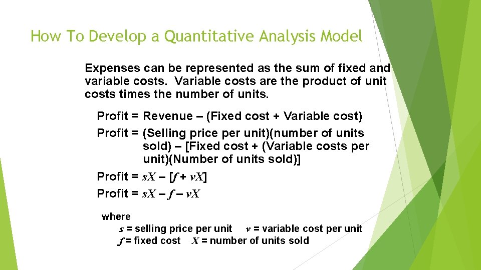
How To Develop a Quantitative Analysis Model Expenses can be represented as the sum of fixed and variable costs. Variable costs are the product of unit costs times the number of units. Profit = Revenue – (Fixed cost + Variable cost) Profit = (Selling price per unit)(number of units sold) – [Fixed cost + (Variable costs per unit)(Number of units sold)] Profit = s. X – [f + v. X] Profit = s. X – f – v. X where s = selling price per unit v = variable cost per unit f = fixed cost X = number of units sold

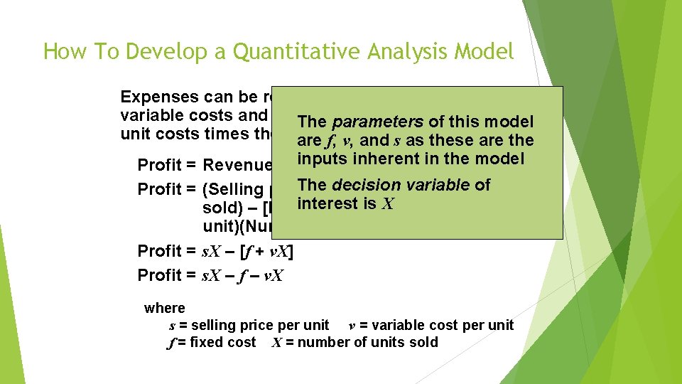
How To Develop a Quantitative Analysis Model Expenses can be represented as the sum of fixed and variable costs are the product of The parameters of this model unit costs times the number units are f, v, of and s as these are the inputscost inherent in the cost) model Profit = Revenue – (Fixed + Variable The decision variable Profit = (Selling price per unit)(number of of units interest X sold) – [Fixed cost +is(Variable costs per unit)(Number of units sold)] Profit = s. X – [f + v. X] Profit = s. X – f – v. X where s = selling price per unit v = variable cost per unit f = fixed cost X = number of units sold

Advantages of Mathematical Modeling 1. Models can accurately represent reality. 2. Models can help a decision maker formulate problems. 3. Models can give us insight and information. 4. Models can save time and money in decision making and problem solving. 5. A model may be the only way to solve large or complex problems in a timely fashion. 6. A model can be used to communicate problems and solutions to others.

Models Categorized by Risk Mathematical models that do not involve risk are called deterministic models. All of the values used in the model are known with complete certainty. Mathematical models that involve risk, chance, or uncertainty are called probabilistic models. Values used in the model are estimates based on probabilities.

Computers and Spreadsheet Models QM for Windows n An easy to use decision support system for use in POM and QM courses n This is the main menu of quantitative models Program 1. 1

PROBABILITY? Probability is a numerical statement about the likelihood that an event will occur.

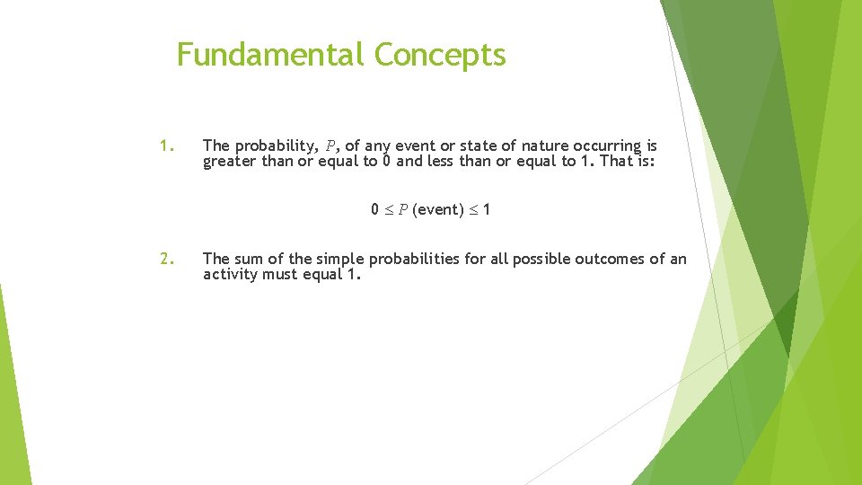
Fundamental Concepts 1. The probability, P, of any event or state of nature occurring is greater than or equal to 0 and less than or equal to 1. That is: 0 P (event) 1 2. The sum of the simple probabilities for all possible outcomes of an activity must equal 1.

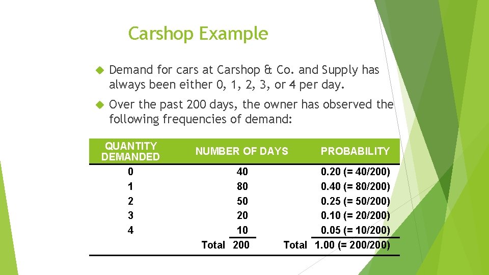
Carshop Example Demand for cars at Carshop & Co. and Supply has always been either 0, 1, 2, 3, or 4 per day. Over the past 200 days, the owner has observed the following frequencies of demand: QUANTITY DEMANDED 0 1 2 3 4 NUMBER OF DAYS 40 80 50 20 10 Total 200 PROBABILITY 0. 20 (= 40/200) 0. 40 (= 80/200) 0. 25 (= 50/200) 0. 10 (= 20/200) 0. 05 (= 10/200) Total 1. 00 (= 200/200)

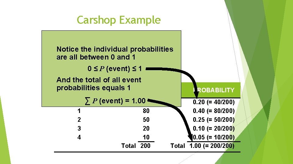
Carshop Example Notice the individual probabilities are all between 0 and 1 0 ≤ P (event) ≤ 1 And the total of all event QUANTITY equals 1 probabilities NUMBER OF DAYS DEMANDED 0 ∑P 1 2 3 4 (event) = 1. 0040 80 50 20 10 Total 200 PROBABILITY 0. 20 (= 40/200) 0. 40 (= 80/200) 0. 25 (= 50/200) 0. 10 (= 20/200) 0. 05 (= 10/200) Total 1. 00 (= 200/200)

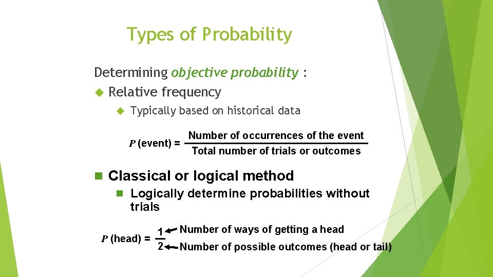
Types of Probability Determining objective probability : Relative frequency Typically based on historical data Number of occurrences of the event P (event) = Total number of trials or outcomes n Classical or logical method n Logically determine probabilities without trials 1 P (head) = 2 Number of ways of getting a head Number of possible outcomes (head or tail)

Types of Probability Subjective probability is based on the experience and judgment of the person making the estimate. Opinion polls Judgment Delphi of experts method

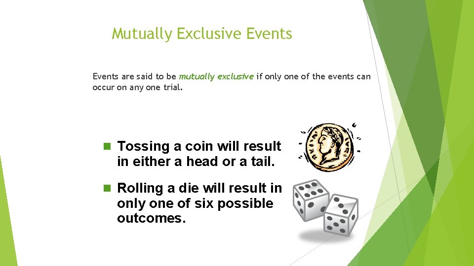
Mutually Exclusive Events are said to be mutually exclusive if only one of the events can occur on any one trial. n Tossing a coin will result in either a head or a tail. n Rolling a die will result in only one of six possible outcomes.

Collectively Exhaustive Events are said to be collectively exhaustive if the list of outcomes includes every possible outcome. Both heads and tails as possible outcomes of coin flips. All six possible outcomes of the roll of a die. OUTCOME OF ROLL 1 2 3 4 5 6 PROBABILITY 1/ 6 1/ 6 Total 1

Drawing a Card Draw one card from a deck of 52 playing cards P (drawing a 7) = 4/52 = 1/13 P (drawing a heart) = 13/52 = 1/4 n These two events are not mutually exclusive since a 7 of hearts can be drawn n These two events are not collectively exhaustive since there are other cards in the deck besides 7 s and hearts

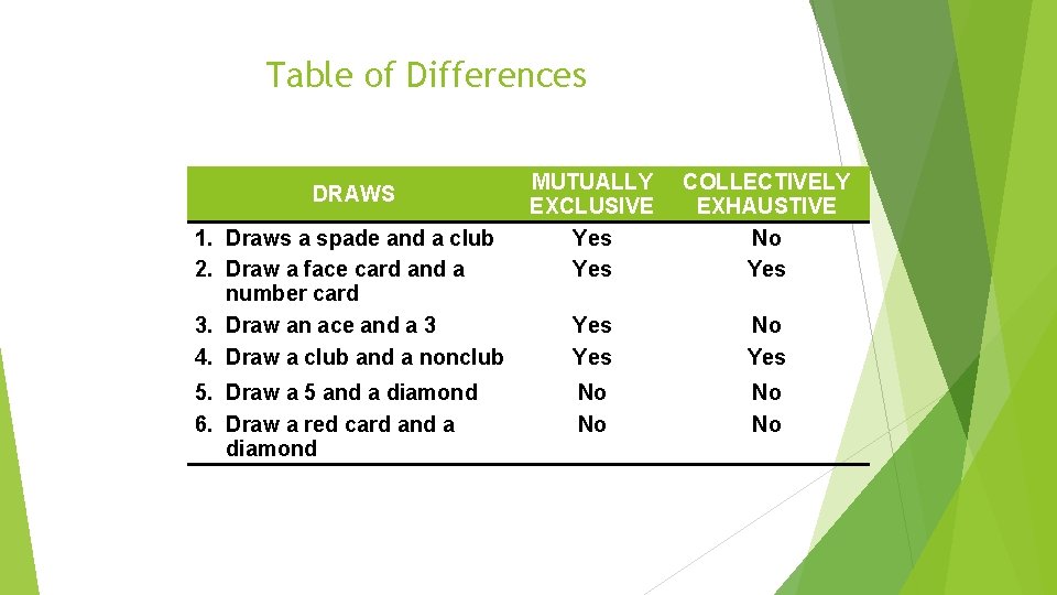
Table of Differences DRAWS 1. Draws a spade and a club 2. Draw a face card and a number card 3. Draw an ace and a 3 4. Draw a club and a nonclub 5. Draw a 5 and a diamond 6. Draw a red card and a diamond MUTUALLY EXCLUSIVE Yes COLLECTIVELY EXHAUSTIVE No Yes Yes No No

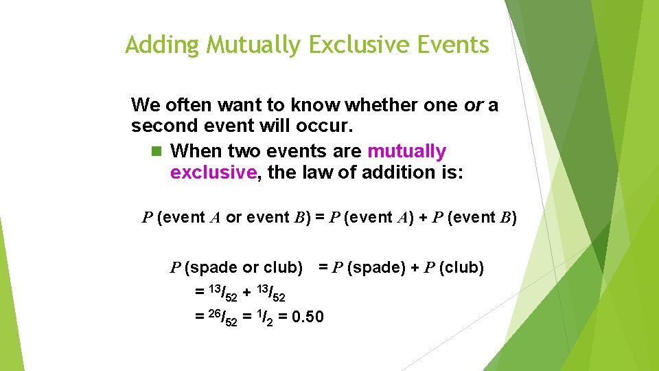
Adding Mutually Exclusive Events We often want to know whether one or a second event will occur. n When two events are mutually exclusive, the law of addition is: P (event A or event B) = P (event A) + P (event B) P (spade or club) = P (spade) + P (club) = 13/52 + 13/52 = 26/52 = 1/2 = 0. 50

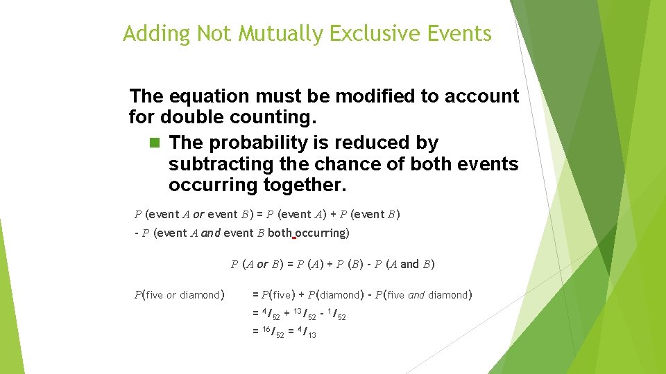
Adding Not Mutually Exclusive Events The equation must be modified to account for double counting. n The probability is reduced by subtracting the chance of both events occurring together. P (event A or event B) = P (event A) + P (event B) – P (event A and event B both occurring) P (A or B) = P (A) + P (B) – P (A and B) P(five or diamond) = P(five) + P(diamond) – P(five and diamond) = 4/52 + 13/52 – 1/52 = 16/52 = 4/13

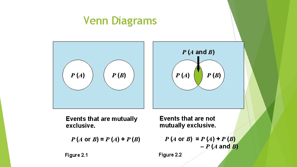
Venn Diagrams P (A and B) P (A) P (B) Events that are mutually exclusive. P (A or B) = P (A) + P (B) Figure 2. 1 P (A) P (B) Events that are not mutually exclusive. P (A or B) = P (A) + P (B) – P (A and B) Figure 2. 2

Statistically Independent Events may be either independent or dependent. For independent events, the occurrence of one event has no effect on the probability of occurrence of the second event.

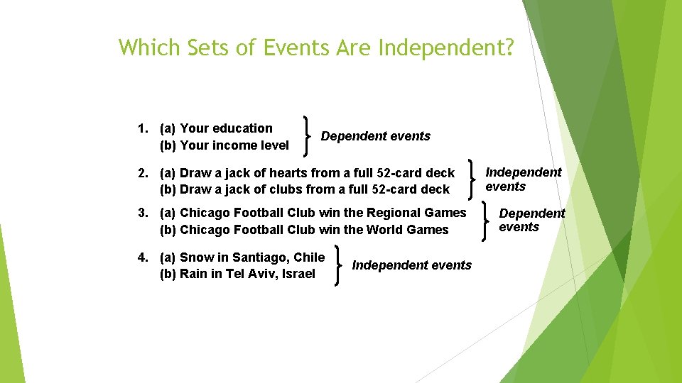
Which Sets of Events Are Independent? 1. (a) Your education (b) Your income level Dependent events 2. (a) Draw a jack of hearts from a full 52 -card deck (b) Draw a jack of clubs from a full 52 -card deck 3. (a) Chicago Football Club win the Regional Games (b) Chicago Football Club win the World Games 4. (a) Snow in Santiago, Chile (b) Rain in Tel Aviv, Israel Independent events Dependent events

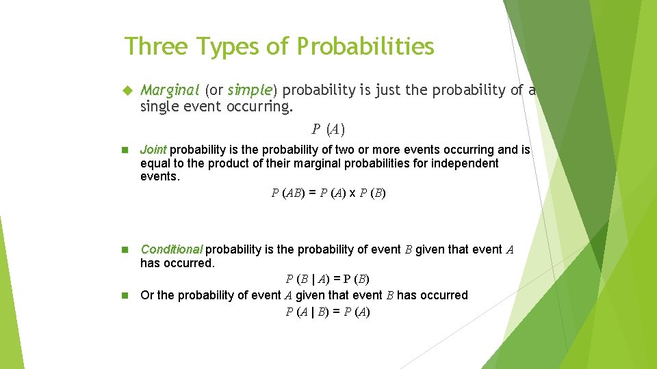
Three Types of Probabilities Marginal (or simple) simple probability is just the probability of a single event occurring. P (A) n Joint probability is the probability of two or more events occurring and is equal to the product of their marginal probabilities for independent events. P (AB) = P (A) x P (B) n Conditional probability is the probability of event B given that event A has occurred. P (B | A) = P (B) n Or the probability of event A given that event B has occurred P (A | B) = P (A)

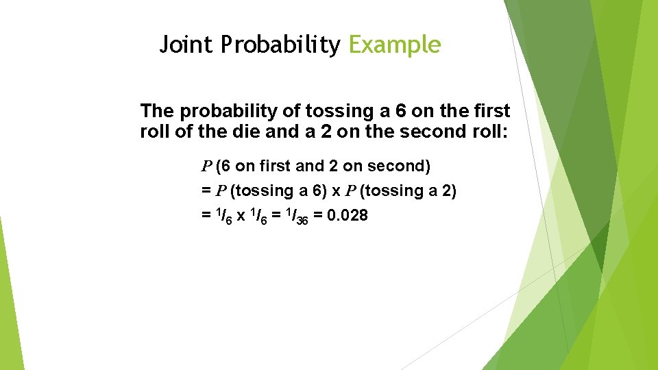
Joint Probability Example The probability of tossing a 6 on the first roll of the die and a 2 on the second roll: P (6 on first and 2 on second) = P (tossing a 6) x P (tossing a 2) = 1/6 x 1/6 = 1/36 = 0. 028

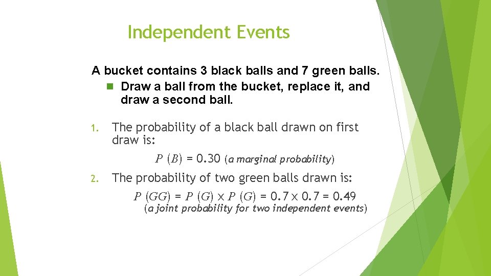
Independent Events A bucket contains 3 black balls and 7 green balls. n Draw a ball from the bucket, replace it, and draw a second ball. 1. The probability of a black ball drawn on first draw is: P (B) = 0. 30 (a marginal probability) 2. The probability of two green balls drawn is: P (GG) = P (G) x P (G) = 0. 7 x 0. 7 = 0. 49 (a joint probability for two independent events)

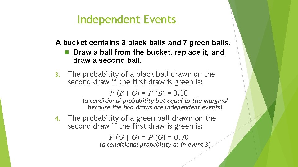
Independent Events A bucket contains 3 black balls and 7 green balls. n Draw a ball from the bucket, replace it, and draw a second ball. 3. The probability of a black ball drawn on the second draw if the first draw is green is: P (B | G) = P (B) = 0. 30 (a conditional probability but equal to the marginal because the two draws are independent events) 4. The probability of a green ball drawn on the second draw if the first draw is green is: P (G | G) = P (G) = 0. 70 (a conditional probability as in event 3)

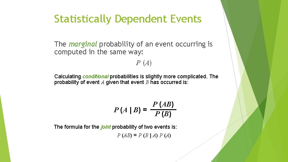
Statistically Dependent Events The marginal probability of an event occurring is computed in the same way: P (A) Calculating conditional probabilities is slightly more complicated. The probability of event A given that event B has occurred is: P (AB) P (A | B) = P (B) The formula for the joint probability of two events is: P (AB) = P (B | A) P (A)

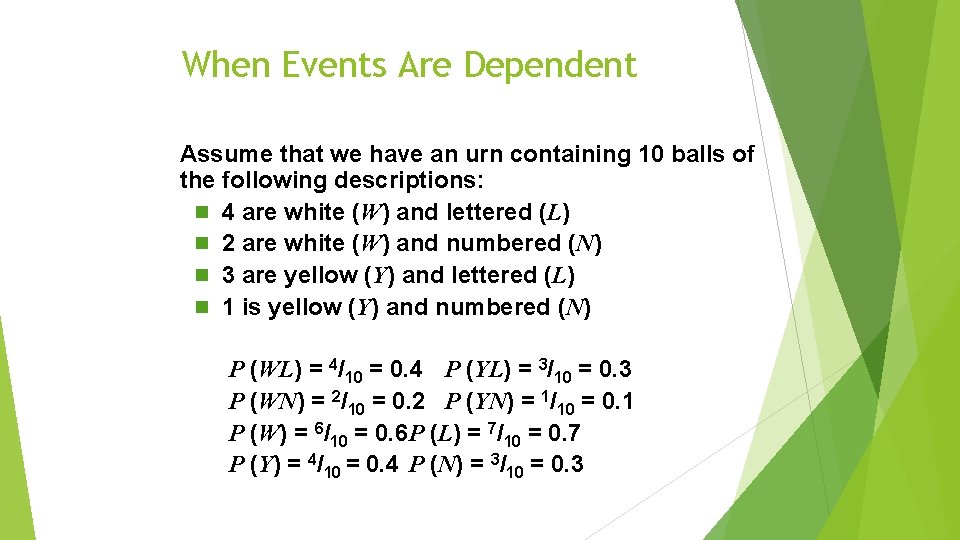
When Events Are Dependent Assume that we have an urn containing 10 balls of the following descriptions: n 4 are white (W) and lettered (L) n 2 are white (W) and numbered (N) n 3 are yellow (Y) and lettered (L) n 1 is yellow (Y) and numbered (N) P (WL) = 4/10 = 0. 4 P (YL) = 3/10 = 0. 3 P (WN) = 2/10 = 0. 2 P (YN) = 1/10 = 0. 1 P (W) = 6/10 = 0. 6 P (L) = 7/10 = 0. 7 P (Y) = 4/10 = 0. 4 P (N) = 3/10 = 0. 3

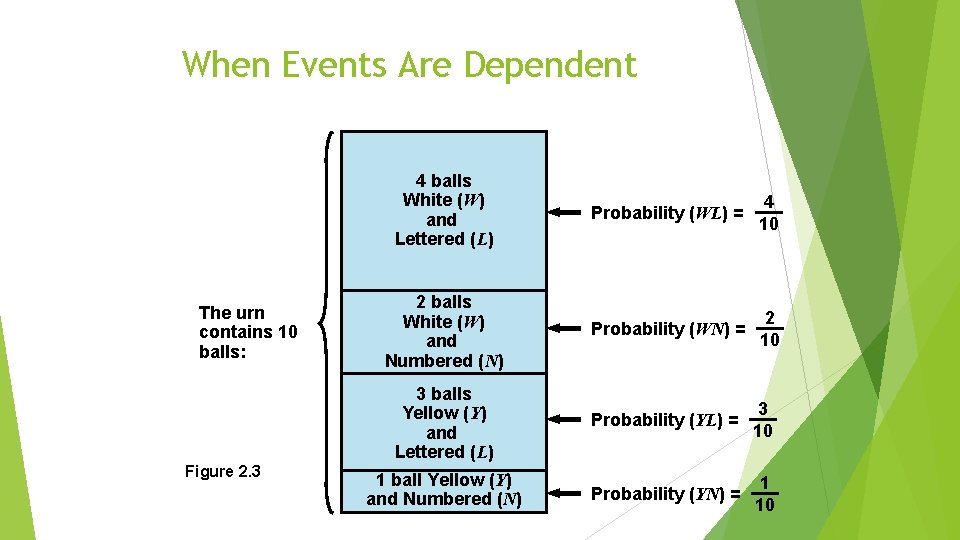
When Events Are Dependent The urn contains 10 balls: Figure 2. 3 4 balls White (W) and Lettered (L) Probability (WL) = 4 10 2 balls White (W) and Numbered (N) Probability (WN) = 2 10 3 balls Yellow (Y) and Lettered (L) Probability (YL) = 3 10 1 ball Yellow (Y) and Numbered (N) Probability (YN) = 1 10

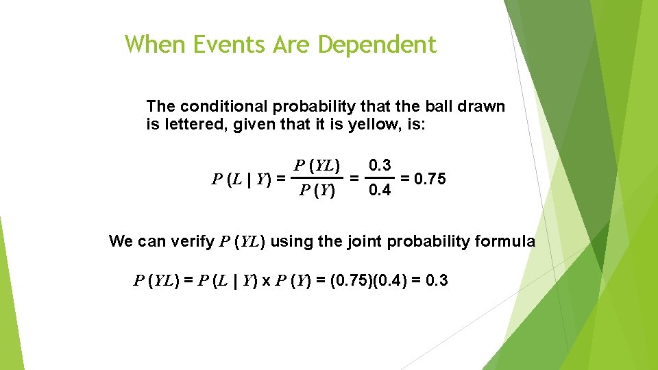
When Events Are Dependent The conditional probability that the ball drawn is lettered, given that it is yellow, is: P (YL) 0. 3 P (L | Y) = = = 0. 75 P (Y) 0. 4 We can verify P (YL) using the joint probability formula P (YL) = P (L | Y) x P (Y) = (0. 75)(0. 4) = 0. 3

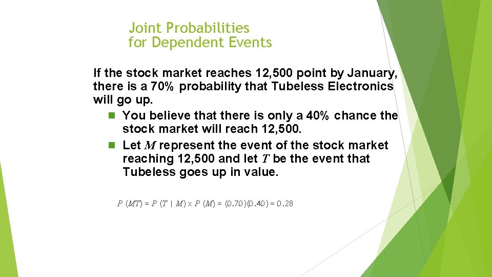
Joint Probabilities for Dependent Events If the stock market reaches 12, 500 point by January, there is a 70% probability that Tubeless Electronics will go up. n You believe that there is only a 40% chance the stock market will reach 12, 500. n Let M represent the event of the stock market reaching 12, 500 and let T be the event that Tubeless goes up in value. P (MT) = P (T | M) x P (M) = (0. 70)(0. 40) = 0. 28

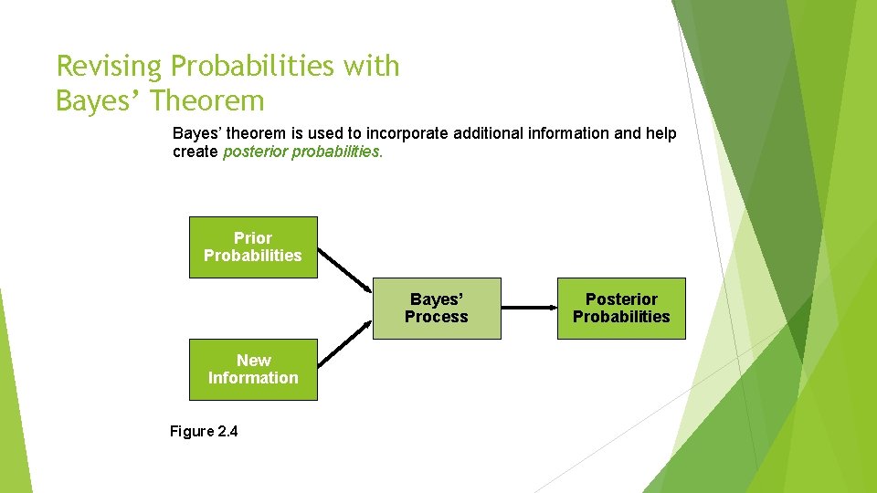
Revising Probabilities with Bayes’ Theorem Bayes’ theorem is used to incorporate additional information and help create posterior probabilities. Prior Probabilities Bayes’ Process New Information Figure 2. 4 Posterior Probabilities

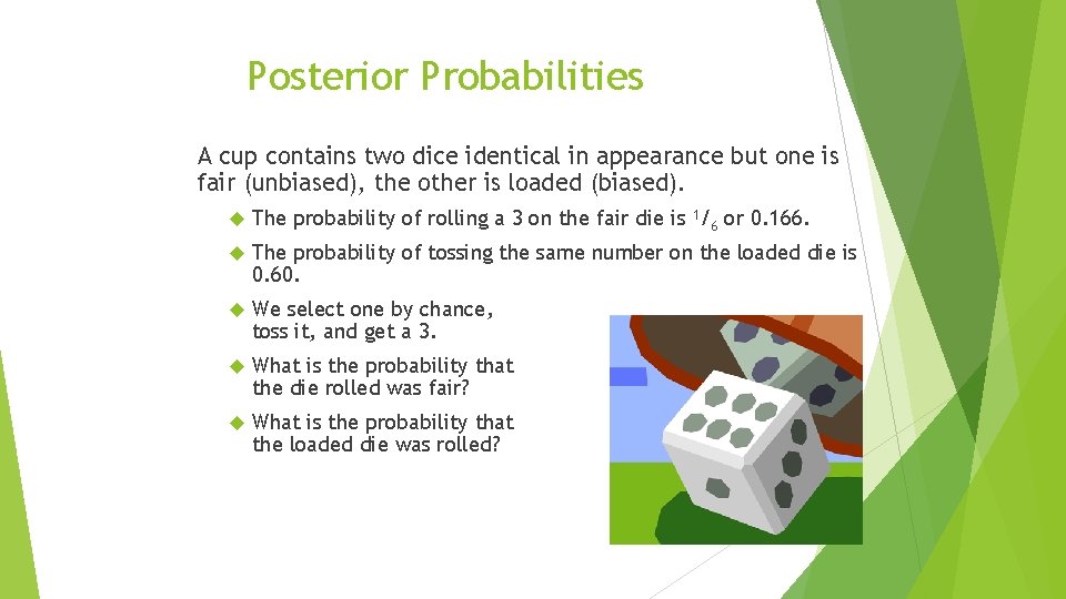
Posterior Probabilities A cup contains two dice identical in appearance but one is fair (unbiased), the other is loaded (biased). The probability of rolling a 3 on the fair die is 1/6 or 0. 166. The probability of tossing the same number on the loaded die is 0. 60. We select one by chance, toss it, and get a 3. What is the probability that the die rolled was fair? What is the probability that the loaded die was rolled?

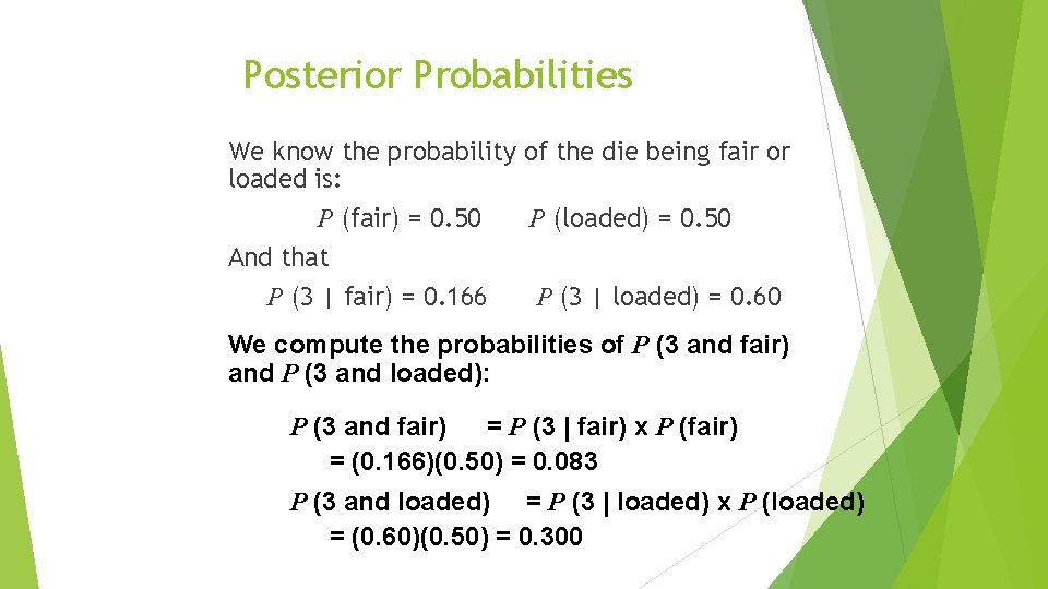
Posterior Probabilities We know the probability of the die being fair or loaded is: P (fair) = 0. 50 P (loaded) = 0. 50 And that P (3 | fair) = 0. 166 P (3 | loaded) = 0. 60 We compute the probabilities of P (3 and fair) and P (3 and loaded): P (3 and fair) = P (3 | fair) x P (fair) = (0. 166)(0. 50) = 0. 083 P (3 and loaded) = P (3 | loaded) x P (loaded) = (0. 60)(0. 50) = 0. 300

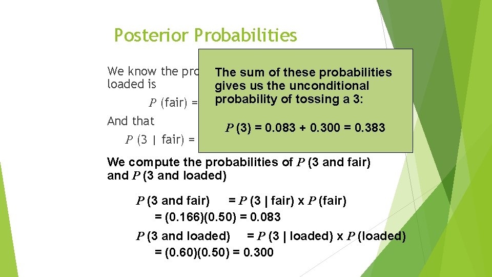
Posterior Probabilities We know the probability of the being fair or The sum of die these probabilities loaded is gives us the unconditional probability of tossing P (fair) = 0. 50 P (loaded) = 0. 50 a 3: And that P (3) = 0. 083 + 0. 300 = 0. 383 P (3 | fair) = 0. 166 P (3 | loaded) = 0. 60 We compute the probabilities of P (3 and fair) and P (3 and loaded) P (3 and fair) = P (3 | fair) x P (fair) = (0. 166)(0. 50) = 0. 083 P (3 and loaded) = P (3 | loaded) x P (loaded) = (0. 60)(0. 50) = 0. 300

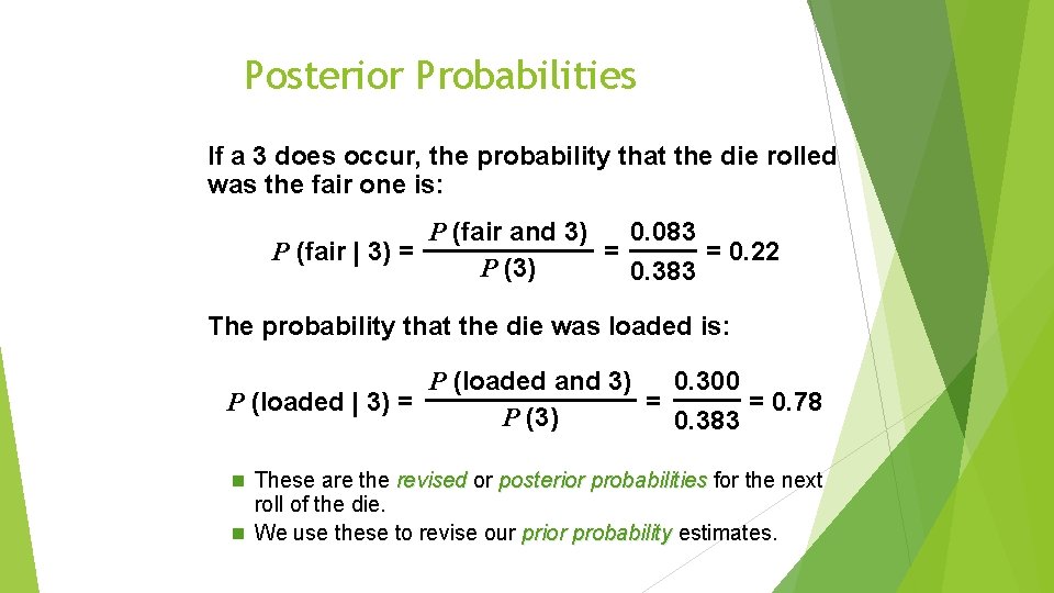
Posterior Probabilities If a 3 does occur, the probability that the die rolled was the fair one is: P (fair and 3) 0. 083 P (fair | 3) = = = 0. 22 P (3) 0. 383 The probability that the die was loaded is: P (loaded and 3) 0. 300 P (loaded | 3) = = = 0. 78 P (3) 0. 383 n These are the revised or posterior probabilities for the next roll of the die. n We use these to revise our prior probability estimates.

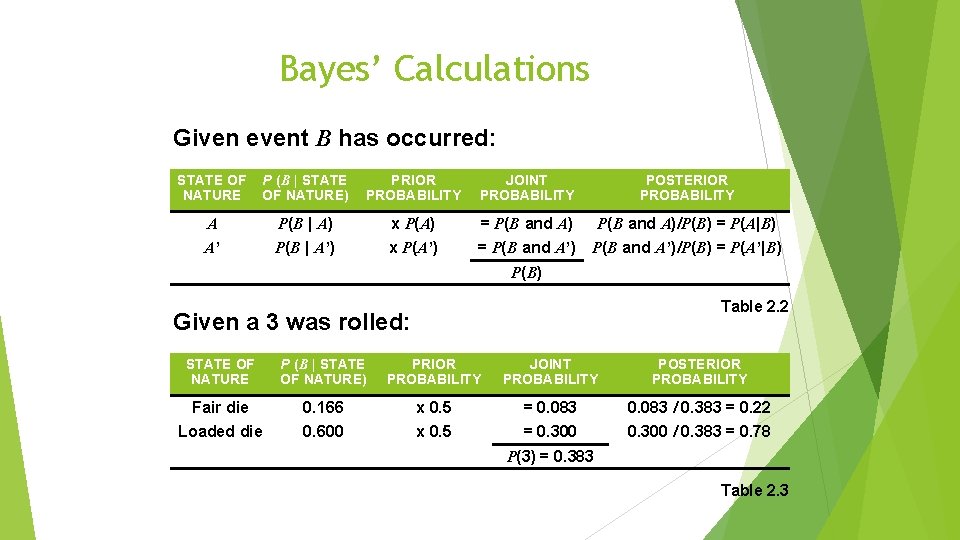
Bayes’ Calculations Given event B has occurred: STATE OF NATURE P (B | STATE OF NATURE) PRIOR PROBABILITY JOINT PROBABILITY POSTERIOR PROBABILITY A P(B | A) x P(A) = P(B and A)/P(B) = P(A|B) A’ P(B | A’) x P(A’) = P(B and A’)/P(B) = P(A’|B) P(B) Table 2. 2 Given a 3 was rolled: STATE OF NATURE P (B | STATE OF NATURE) PRIOR PROBABILITY JOINT PROBABILITY POSTERIOR PROBABILITY Fair die 0. 166 x 0. 5 = 0. 083 / 0. 383 = 0. 22 Loaded die 0. 600 x 0. 5 = 0. 300 / 0. 383 = 0. 78 P(3) = 0. 383 Table 2. 3

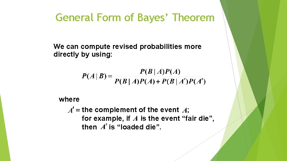
General Form of Bayes’ Theorem We can compute revised probabilities more directly by using: where A¢ = the complement of the event ; for example, if is the event “fair die”, then is “loaded die”.

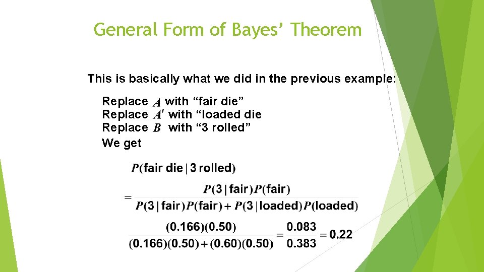
General Form of Bayes’ Theorem This is basically what we did in the previous example: Replace We get with “fair die” with “loaded die with “ 3 rolled”

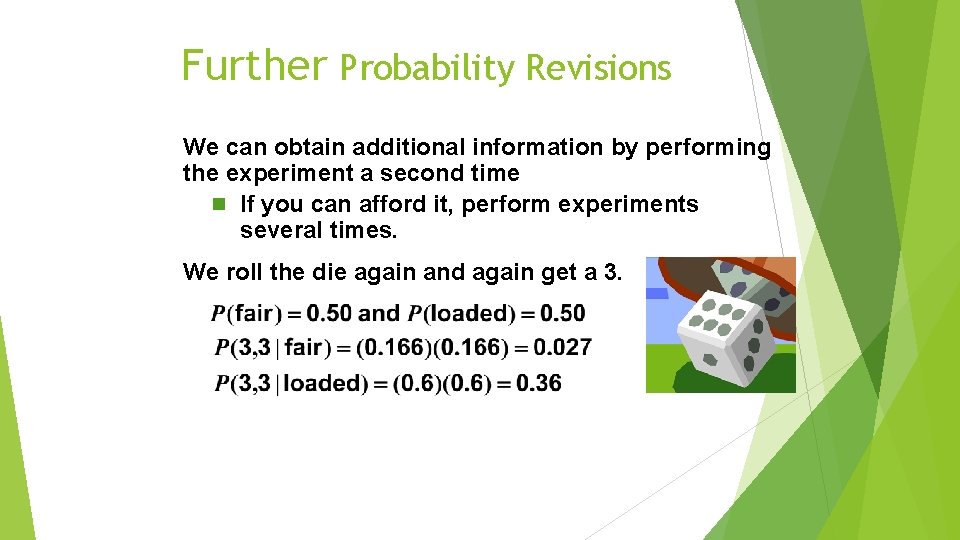
Further Probability Revisions We can obtain additional information by performing the experiment a second time n If you can afford it, perform experiments several times. We roll the die again and again get a 3.

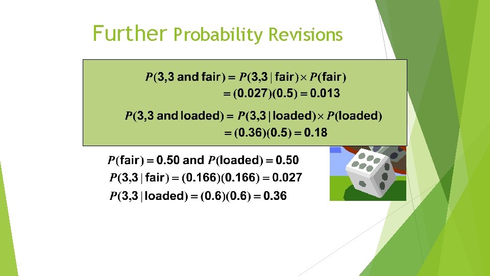
Further Probability Revisions We can obtain additional information by performing the experiment a second time n If you can afford it, perform experiments several times We roll the die again and again get a 3

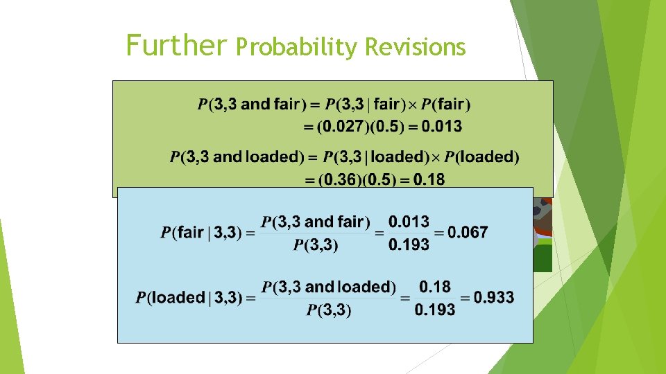
Further Probability Revisions We can obtain additional information by performing the experiment a second time n If you can afford it, perform experiments several times We roll the die again and again get a 3

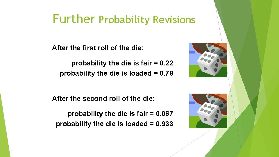
Further Probability Revisions After the first roll of the die: probability the die is fair = 0. 22 probability the die is loaded = 0. 78 After the second roll of the die: probability the die is fair = 0. 067 probability the die is loaded = 0. 933

Random Variables A random variable assigns a real number to every possible outcome or event in an experiment. X = number of refrigerators sold during the day Discrete random variables can assume only a finite or limited set of values. Continuous random variables can assume any one of an infinite set of values.

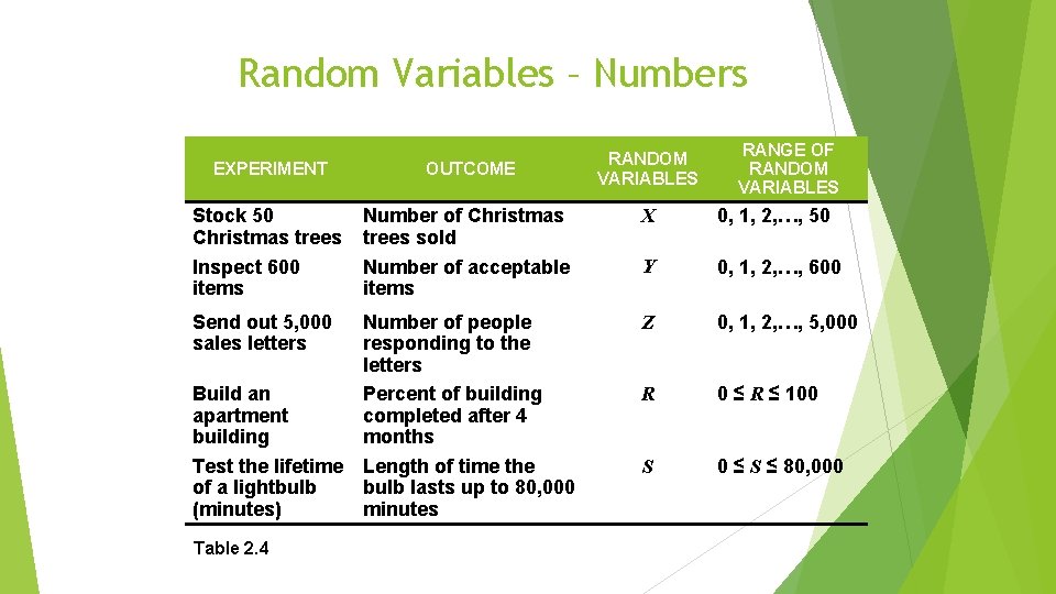
Random Variables – Numbers RANDOM VARIABLES RANGE OF RANDOM VARIABLES EXPERIMENT OUTCOME Stock 50 Christmas trees Inspect 600 items Number of Christmas trees sold Number of acceptable items X 0, 1, 2, …, 50 Y 0, 1, 2, …, 600 Send out 5, 000 sales letters Number of people responding to the letters Percent of building completed after 4 months Length of time the bulb lasts up to 80, 000 minutes Z 0, 1, 2, …, 5, 000 R 0 ≤ R ≤ 100 S 0 ≤ S ≤ 80, 000 Build an apartment building Test the lifetime of a lightbulb (minutes) Table 2. 4

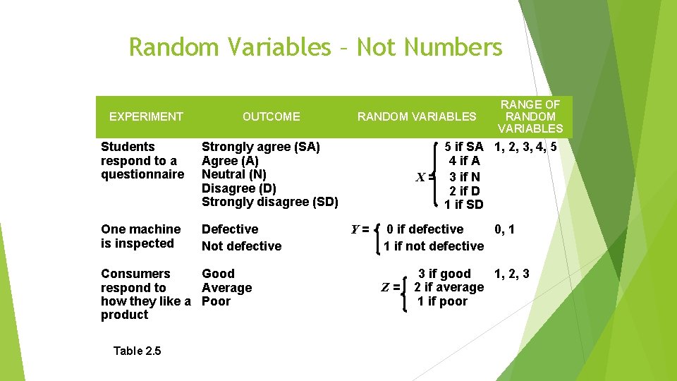
Random Variables – Not Numbers EXPERIMENT OUTCOME Students respond to a questionnaire Strongly agree (SA) Agree (A) Neutral (N) Disagree (D) Strongly disagree (SD) One machine is inspected Defective Not defective Consumers Good respond to Average how they like a Poor product Table 2. 5 RANDOM VARIABLES RANGE OF RANDOM VARIABLES 5 if SA 1, 2, 3, 4, 5 4 if A. . X = 3 if N. . 2 if D. . 1 if SD Y= 0 if defective 0, 1 1 if not defective Z= 3 if good…. 1, 2, 3 2 if average 1 if poor…. .

Probability Distribution of a Discrete Random Variable For discrete random variables a probability is assigned to each event. The students in Pat Shannon’s statistics class have just completed a quiz of five algebra problems. The distribution of correct scores is given in the following table:

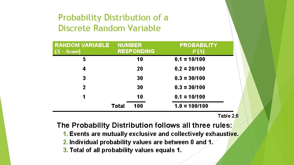
Probability Distribution of a Discrete Random Variable RANDOM VARIABLE (X – Score) 5 NUMBER RESPONDING 10 PROBABILITY P (X) 0. 1 = 10/100 4 20 0. 2 = 20/100 3 30 0. 3 = 30/100 2 30 0. 3 = 30/100 1 10 0. 1 = 10/100 1. 0 = 100/100 Total Table 2. 6 The Probability Distribution follows all three rules: 1. Events are mutually exclusive and collectively exhaustive. 2. Individual probability values are between 0 and 1. 3. Total of all probability values equals 1.

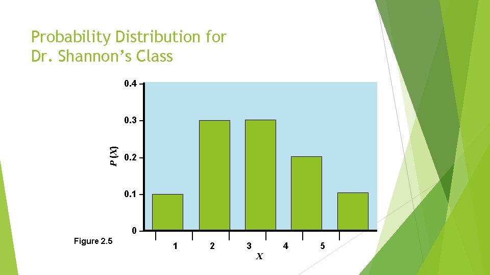
Probability Distribution for Dr. Shannon’s Class 0. 4 – P (X) 0. 3 – 0. 2 – 0. 1 – 0– Figure 2. 5 | | 1 | 2 | 3 | 4 X | 5

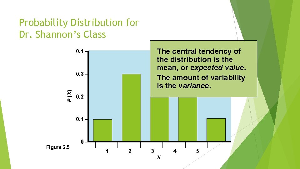
Probability Distribution for Dr. Shannon’s Class The central tendency of the distribution is the mean, or expected value. The amount of variability is the variance. 0. 4 – P (X) 0. 3 – 0. 2 – 0. 1 – Figure 2. 5 0– | | 1 | 2 | 3 | 4 X | 5

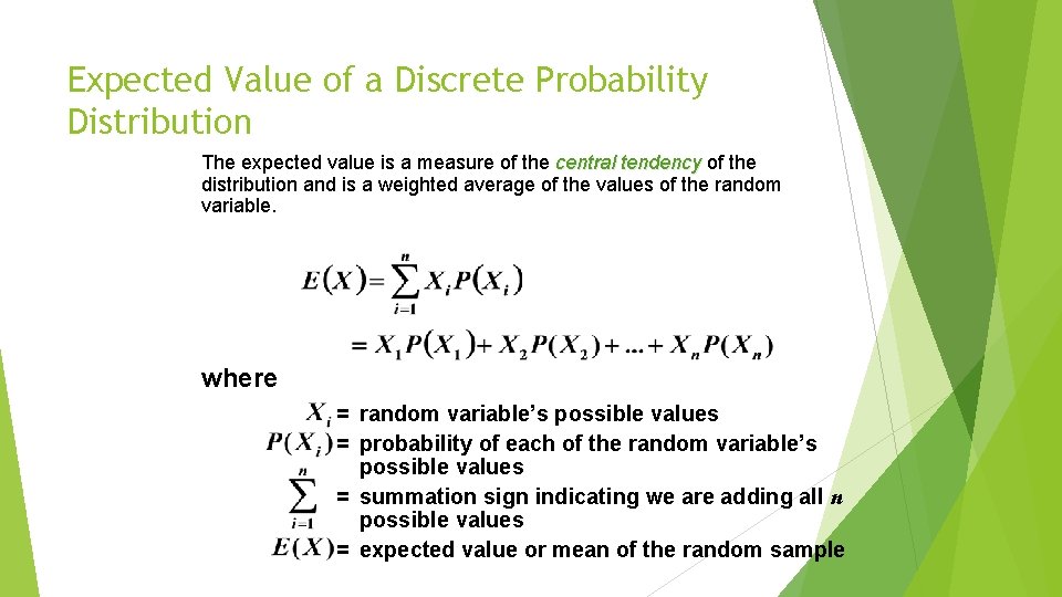
Expected Value of a Discrete Probability Distribution The expected value is a measure of the central tendency of the distribution and is a weighted average of the values of the random variable. where = random variable’s possible values = probability of each of the random variable’s possible values = summation sign indicating we are adding all n possible values = expected value or mean of the random sample

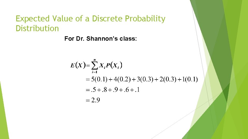
Expected Value of a Discrete Probability Distribution For Dr. Shannon’s class:

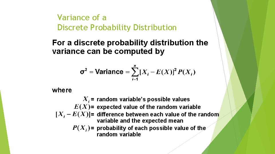
Variance of a Discrete Probability Distribution For a discrete probability distribution the variance can be computed by where = random variable’s possible values = expected value of the random variable = difference between each value of the random variable and the expected mean = probability of each possible value of the random variable

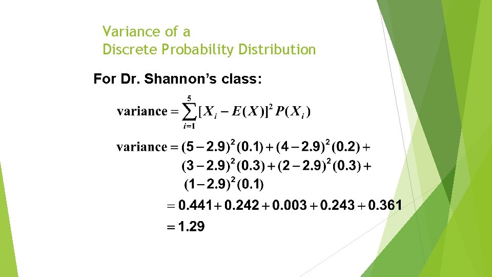
Variance of a Discrete Probability Distribution For Dr. Shannon’s class:

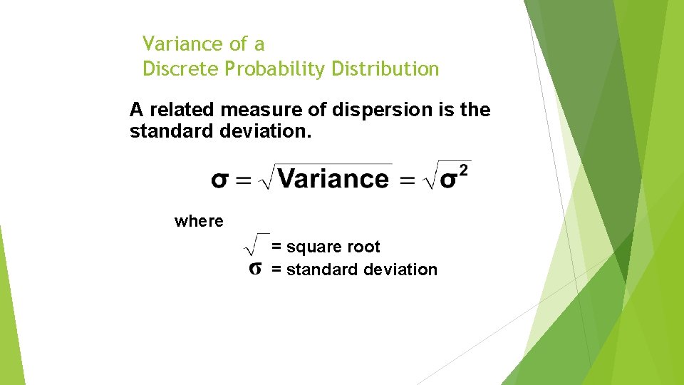
Variance of a Discrete Probability Distribution A related measure of dispersion is the standard deviation. where = square root = standard deviation

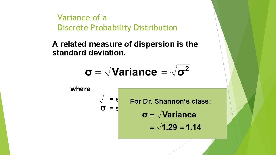
Variance of a Discrete Probability Distribution A related measure of dispersion is the standard deviation. where = square Forroot Dr. Shannon’s class: = standard deviation

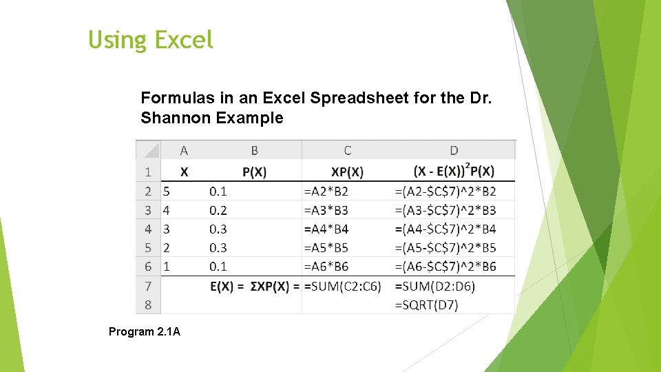
Using Excel Formulas in an Excel Spreadsheet for the Dr. Shannon Example Program 2. 1 A

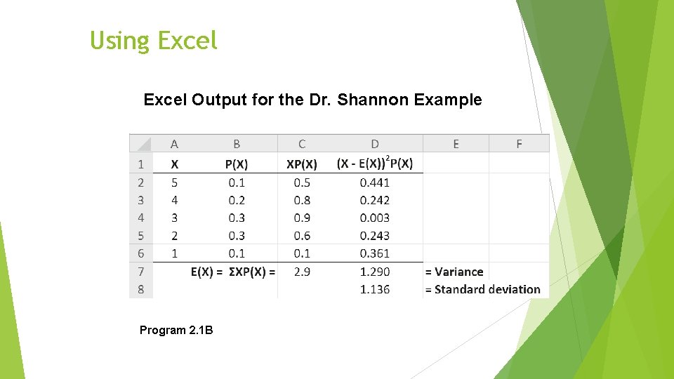
Using Excel Output for the Dr. Shannon Example Program 2. 1 B

Probability Distribution of a Continuous Random Variable Since random variables can take on an infinite number of values, the fundamental rules for continuous random variables must be modified. n The sum of the probability values must still equal 1. n The probability of each individual value of the random variable occurring must equal 0 or the sum would be infinitely large. The probability distribution is defined by a continuous mathematical function called the probability density function or just the probability function. n This is represented by f (X).

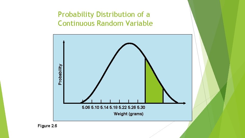
Probability Distribution of a Continuous Random Variable | | | | 5. 06 5. 10 5. 14 5. 18 5. 22 5. 26 5. 30 Weight (grams) Figure 2. 6