BUS 525 Managerial Economics Lecture 4 Theory of
BUS 525: Managerial Economics Lecture 4 Theory of Individual Behavior
Overview I. Consumer Behavior – Indifference Curve Analysis – Consumer Preference Ordering II. Constraints – The Budget Constraint – Changes in Income – Changes in Prices III. Consumer Equilibrium IV. Indifference Curve Analysis & Demand Curves – Individual Demand – Market Demand
Consumer Behavior • Consumer Opportunities – The possible goods and services consumer can afford to consume. • Consumer Preferences – The goods and services consumers actually consume. • You might afford something but actually may not consume something due to personal preference
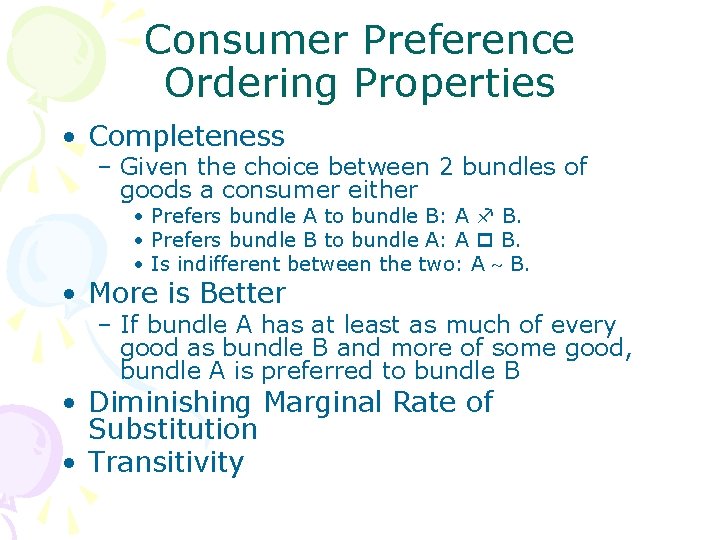
Consumer Preference Ordering Properties • Completeness – Given the choice between 2 bundles of goods a consumer either • Prefers bundle A to bundle B: A B. • Prefers bundle B to bundle A: A B. • Is indifferent between the two: A B. • More is Better – If bundle A has at least as much of every good as bundle B and more of some good, bundle A is preferred to bundle B • Diminishing Marginal Rate of Substitution • Transitivity
Definitions • Indifferent – when a consumer finds two options to be equally satisfactory • Economic “bads” – commodities of which less is preferred to more over all possible ranges of consumption • Economics “goods” – commodities of which more is better than less
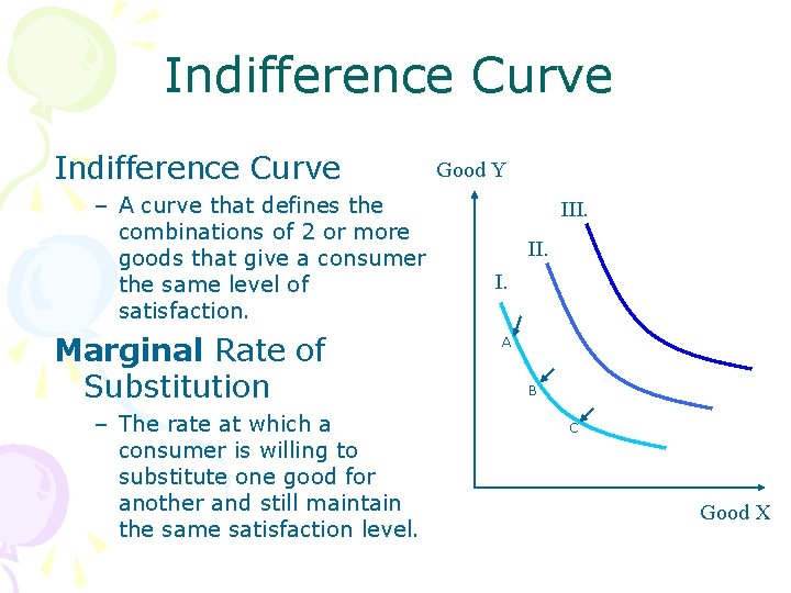
Indifference Curve – A curve that defines the combinations of 2 or more goods that give a consumer the same level of satisfaction. Marginal Rate of Substitution – The rate at which a consumer is willing to substitute one good for another and still maintain the same satisfaction level. Good Y III. I. A B C Good X
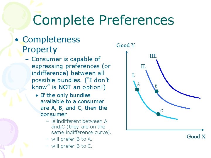
Complete Preferences • Completeness Property – Consumer is capable of expressing preferences (or indifference) between all possible bundles. (“I don’t know” is NOT an option!) • If the only bundles available to a consumer are A, B, and C, then the consumer – is indifferent between A and C (they are on the same indifference curve). – will prefer B to A. – will prefer B to C. Good Y III. I. A B C Good X
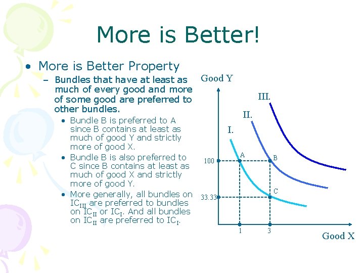
More is Better! • More is Better Property – Bundles that have at least as Good Y much of every good and more of some good are preferred to other bundles. • Bundle B is preferred to A since B contains at least as much of good Y and strictly more of good X. • Bundle B is also preferred to 100 C since B contains at least as much of good X and strictly more of good Y. • More generally, all bundles on 33. 33 ICIII are preferred to bundles on ICII or ICI. And all bundles on ICII are preferred to ICI. III. I. A B C 1 3 Good X
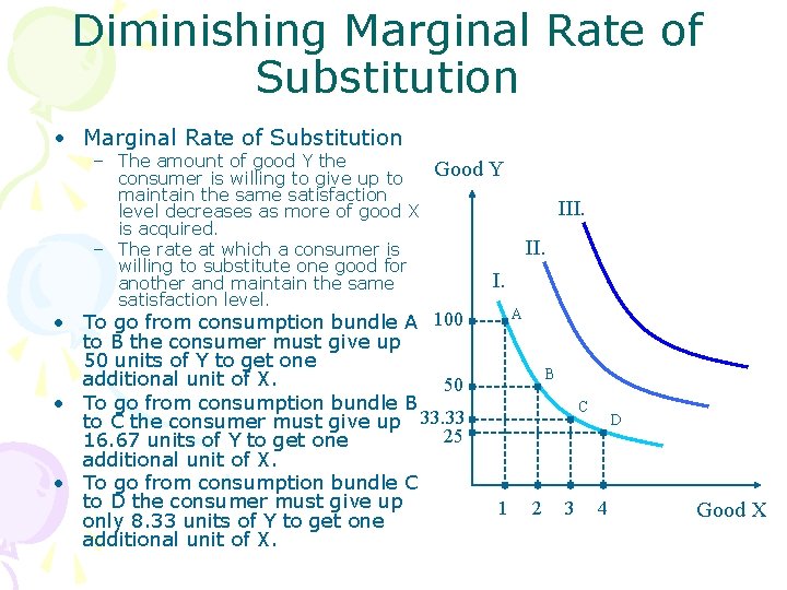
Diminishing Marginal Rate of Substitution • Marginal Rate of Substitution – The amount of good Y the consumer is willing to give up to maintain the same satisfaction level decreases as more of good X is acquired. – The rate at which a consumer is willing to substitute one good for another and maintain the same satisfaction level. Good Y • To go from consumption bundle A 100 to B the consumer must give up 50 units of Y to get one additional unit of X. 50 • To go from consumption bundle B to C the consumer must give up 33. 33 25 16. 67 units of Y to get one additional unit of X. • To go from consumption bundle C to D the consumer must give up only 8. 33 units of Y to get one additional unit of X. III. I. A B C 1 2 3 D 4 Good X
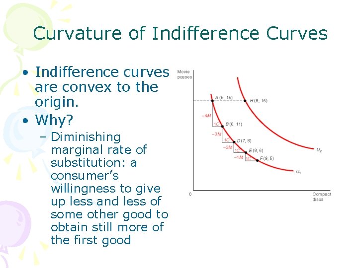
Curvature of Indifference Curves • Indifference curves are convex to the origin. • Why? – Diminishing marginal rate of substitution: a consumer’s willingness to give up less and less of some other good to obtain still more of the first good
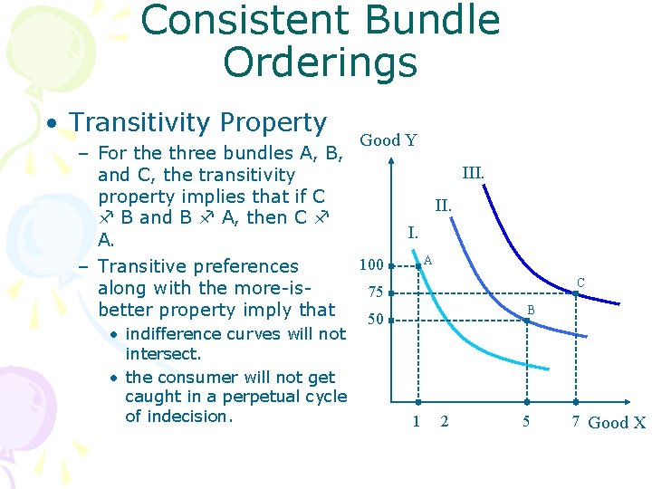
Consistent Bundle Orderings • Transitivity Property Good Y – For the three bundles A, B, III. and C, the transitivity property implies that if C II. B and B A, then C I. A. A 100 – Transitive preferences along with the more-is 75 better property imply that 50 • indifference curves will not intersect. • the consumer will not get caught in a perpetual cycle of indecision. 1 2 C B 5 7 Good X
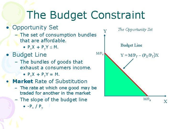
The Budget Constraint • Opportunity Set – The set of consumption bundles that are affordable. Y • Px. X + Py. Y M. • Budget Line M/PY The Opportunity Set Budget Line Y = M/PY – (PX/PY)X – The bundles of goods that exhaust a consumers income. • Px. X + Py. Y = M. • Market Rate of Substitution – The rate at which one good may be traded for another in the market – The slope of the budget line • -Px / Py M/PX X
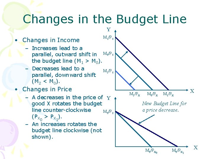
Changes in the Budget Line Y • Changes in Income M 1/PY – Increases lead to a parallel, outward shift in M 0/PY the budget line (M 1 > M 0). – Decreases lead to a M 2/PY parallel, downward shift (M 2 < M 0). • Changes in Price – A decreases in the price of Y good X rotates the budget line counter-clockwise M 0/PY (PX 0 > PX 1). – An increases rotates the budget line clockwise (not shown). M 2/PX M 0/PX X M 1/PX New Budget Line for a price decrease. M 0/PX 0 M 0/PX 1 X
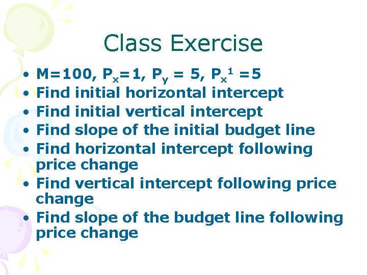
Class Exercise • • • M=100, Px=1, Py = 5, Px 1 =5 Find initial horizontal intercept Find initial vertical intercept Find slope of the initial budget line Find horizontal intercept following price change • Find vertical intercept following price change • Find slope of the budget line following price change
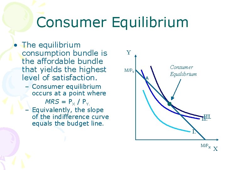
Consumer Equilibrium • The equilibrium consumption bundle is the affordable bundle that yields the highest level of satisfaction. Y M/PY A Consumer Equilibrium – Consumer equilibrium occurs at a point where MRS = PX / PY. – Equivalently, the slope of the indifference curve equals the budget line. III. I. M/PX X
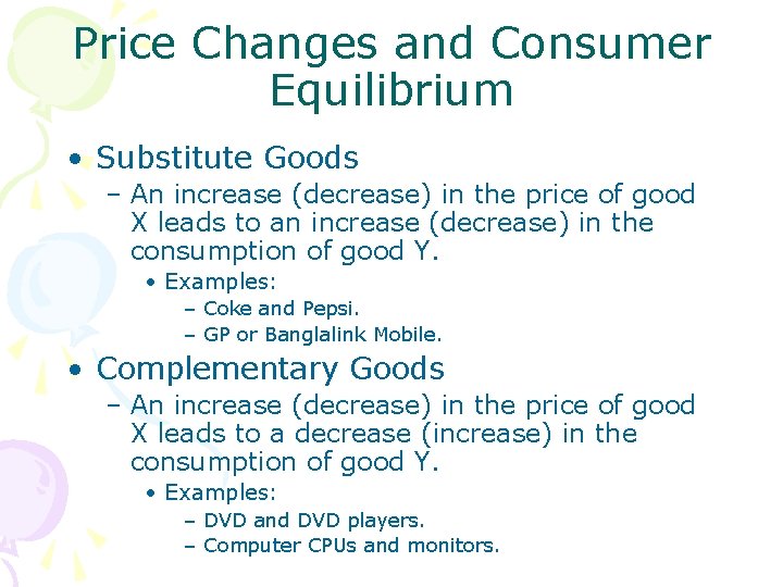
Price Changes and Consumer Equilibrium • Substitute Goods – An increase (decrease) in the price of good X leads to an increase (decrease) in the consumption of good Y. • Examples: – Coke and Pepsi. – GP or Banglalink Mobile. • Complementary Goods – An increase (decrease) in the price of good X leads to a decrease (increase) in the consumption of good Y. • Examples: – DVD and DVD players. – Computer CPUs and monitors.
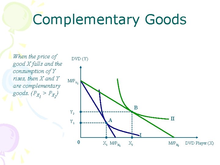
Complementary Goods When the price of good X falls and the consumption of Y rises, then X and Y are complementary goods. (PX 1 > PX 2) DVD (Y) M/PY 1 B Y 2 II A Y 1 I 0 X 1 M/PX 1 X 2 M/PX 2 DVD Player (X)
Income Changes and Consumer Equilibrium • Normal Goods – Good X is a normal good if an increase (decrease) in income leads to an increase (decrease) in its consumption. • Inferior Goods – Good X is an inferior good if an increase (decrease) in income leads to a decrease (increase) in its consumption.
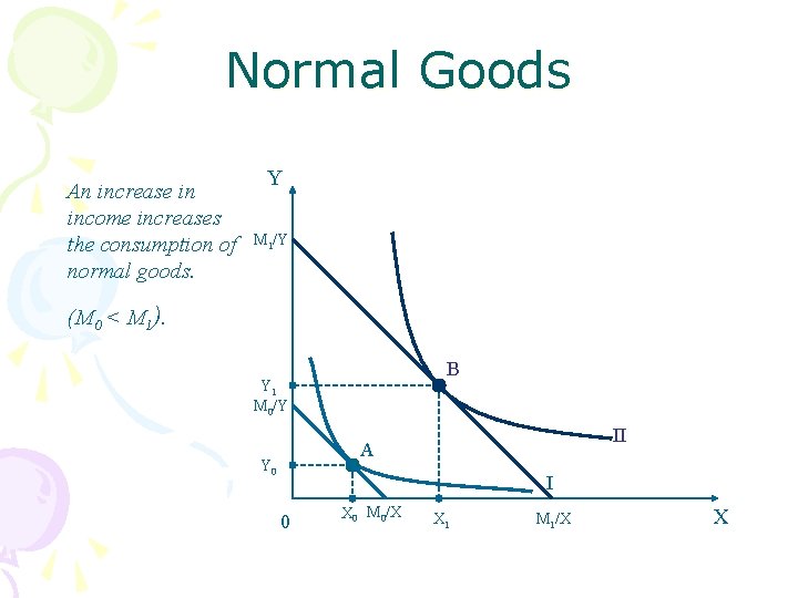
Normal Goods An increase in income increases the consumption of normal goods. Y M 1/Y (M 0 < M 1). B Y 1 M 0/Y II A Y 0 I 0 X 0 M 0/X X 1 M 1/X X
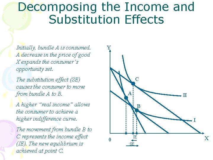
Decomposing the Income and Substitution Effects Initially, bundle A is consumed. A decrease in the price of good X expands the consumer’s opportunity set. Y C The substitution effect (SE) causes the consumer to move from bundle A to B. A II A higher “real income” allows the consumer to achieve a higher indifference curve. The movement from bundle B to C represents the income effect (IE). The new equilibrium is achieved at point C. B I 0 IE SE X
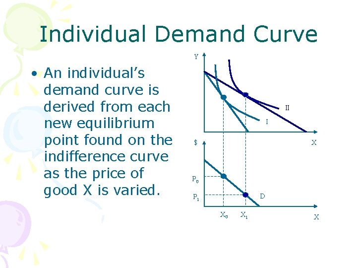
Individual Demand Curve Y • An individual’s demand curve is derived from each new equilibrium point found on the indifference curve as the price of good X is varied. II I X $ P 0 D P 1 X 0 X 1 X
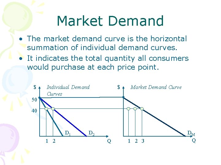
Market Demand • The market demand curve is the horizontal summation of individual demand curves. • It indicates the total quantity all consumers would purchase at each price point. $ 50 Individual Demand Curves $ Market Demand Curve 40 D 1 1 2 D 2 Q 1 2 3 DM Q
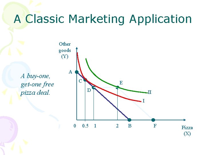
A Classic Marketing Application Other goods (Y) A buy-one, get-one free pizza deal. A C E D II I 0 0. 5 1 2 B F Pizza (X)
Conclusion • Indifference curve properties reveal information about consumers’ preferences between bundles of goods. – Completeness. – More is better. – Diminishing marginal rate of substitution. – Transitivity. • Indifference curves along with price changes determine individuals’ demand curves. • Market demand is the horizontal summation of individuals’ demands.
- Slides: 24