Building useful models Some new developments and easily

Building useful models: Some new developments and easily avoidable errors Michael Babyak, Ph. D
 Y")
What is a model ? Y = f(x 1, x 2, x 3…xn) Y = a + b 1 x 1 + b 2 x 2…bnxn Y = e a + b 1 x 1 + b 2 x 2…bnxn

“All models are wrong, some are useful” -- George Box • A useful model is – Not very biased – Interpretable – Replicable (predicts in a new sample)

Some Premises • “Statistics” is a cumulative, evolving field • Newer is not necessarily better, but should be entertained in the context of the scientific question at hand • Data analytic practice resides along a continuum, from exploratory to confirmatory. Both are important, but the difference has to be recognized. • There’s no substitute for thinking about the problem

Statistics is a cumulative, evolving field: How do we know this stuff? • Theory • Simulation

Concept of Simulation Y = b X + error bs 1 bs 2 bs 3 bs 4 …………………. bsk-1 bsk

Concept of Simulation Y = b X + error bs 1 bs 2 bs 3 bs 4 …………………. bsk-1 Evaluate bsk

Simulation Example Y =. 4 X + error bs 1 bs 2 bs 3 bs 4 …………………. bsk-1 bsk

Simulation Example Y =. 4 X + error bs 1 bs 2 bs 3 bs 4 …………………. bsk-1 Evaluate bsk

True Model: Y =. 4*x 1 + e

Ingredients of a Useful Model Correct probability model Based on theory Good measures/no loss of information Comprehensive Parsimonious Tested fairly Flexible Useful Model

Correct Model • Gaussian: General Linear Model • Multiple linear regression • Binary (or ordinal): Generalized Linear Model • Logistic Regression • Proportional Odds/Ordinal Logistic • Time to event: • Cox Regression or parametric survival models

Generalized Linear Model Normal Binary/Binomial Count, heavy skew, Lots of zeros General Linear Model/ Logistic Regression Poisson, ZIP, negbin, gamma Linear Regression ANOVA/t-test ANCOVA Chi-square Regression w/ Transformed DV Can be applied to clustered (e. g, repeated measures data)

Factor Analytic Family Structural Equation Models Latent Variable Models Partial Least Squares (Confirmatory Factor Analysis) Common Factor Analysis Multiple regression Principal Components

Use Theory • Theory and expert information are critical in helping sift out artifact • Numbers can look very systematic when the are in fact random – http: //www. tufts. edu/~gdallal/multtest. htm

Measure well §Adequate range §Representative values §Watch for ceiling/floor effects

Using all the information §Preserving cases in data sets with missing data §Conventional approaches: §Use only complete case §Fill in with mean or median §Use a missing data indicator in the model

Missing Data • Imputation or related approaches are almost ALWAYS better than deleting incomplete cases • Multiple Imputation • Full Information Maximum Likelihood

Multiple Imputation

Modern Missing Data Techniques § Preserve more information from original sample § Incorporate uncertainty about missingness into final estimates § Produce better estimates of population (true) values

Don’t throw waste information from variables • Use all the information about the variables of interest • Don’t create “clinical cutpoints” before modeling • Model with ALL the data first, then use prediction to make decisions about cutpoints
 • Convoluted Reasoning")
Dichotomizing for Convenience = Dubious Practice (C. R. A. P. *) • Convoluted Reasoning and Anti-intellectual Pomposity • Streiner & Norman: Biostatistics: The Bare Essentials

Implausible measurement assumption “not depressed” “depressed” AB Depression score C

Loss of power http: //psych. colorado. edu/~mcclella/Median. Split/ Sometimes through sampling error You can get a ‘lucky cut. ’ http: //www. bolderstats. com/jmsl/doc/median. Split. html

Dichotomization, by definition, reduces the magnitude of the estimate by a minimum of about 30% Dear Project Officer, In order to facilitate analysis and interpretation, we have decided to throw away about 30% of our data. Even though this will waste about 3 or 4 hundred thousand dollars worth of subject recruitment and testing money, we are confident that you will understand. Sincerely, Dick O. Tomi, Ph. D Prof. Richard Obediah Tomi, Ph. D

Power to detect non-zero b-weight when x is continuous versus dichotomized True model: y =. 4 x + e

Dichotomizing will obscure non-linearity Low High CESD Score

Dichotomizing will obscure non-linearity: Same data as previous slide modeled continuously

Type I error rates for the relation between x 2 and y after dichotomizing two continuous predictors. Maxwell and Delaney calculated the effect of dichotomizing two continuous predictors as a function of the correlation between them. The true model is y =. 5 x 1 + 0 x 2, where all variables are continuous. If x 1 and x 2 are dichotomized, the error rate for the relation between x 2 and y increases as the correlation between x 1 and x 2 increases. Correlation between x 1 and x 2 N 0 . 3 . 5 . 7 50 . 05 . 06 . 08 . 10 100 . 05 . 08 . 12 . 18 200 . 05 . 10 . 19 . 31

Is it ever a good idea to categorize quantitatively measured variables? • Yes: – when the variable is truly categorical – for descriptive/presentational purposes – for hypothesis testing, if enough categories are made. • However, using many categories can lead to problems of multiple significance tests and still run the risk of misclassification

CONCLUSIONS • Cutting: – Doesn’t always make measurement sense – Almost always reduces power – Can fool you with too much power in some instances – Can completely miss important features of the underlying function • Modern computing/statistical packages can “handle” continuous variables • Want to make good clinical cutpoints? Model first, decide on cuts afterward.

Sample size and the problem of underfitting vs overfitting • Model assumption is that “ALL” relevant variables be included—the “antiparsimony principle” • Tempered by fact that estimating too many unknowns with too little data will yield junk

Sample Size Requirements • Linear regression – minimum of N = 50 + 8: predictor (Green, 1990) • Logistic Regression – Minimum of N = 10 -15/predictor among smallest group (Peduzzi et al. , 1990 a) • Survival Analysis – Minimum of N = 10 -15/predictor (Peduzzi et al. , 1990 b)

Consequences of inadequate sample size • Lack of power for individual tests • Unstable estimates • Spurious good fit—lots of unstable estimates will produce spurious ‘goodlooking’ (big) regression coefficients

All-noise, but good fit R-squares from a population model of completelyrandom variables Events per predictor ratio

Simulation: number of events/predictor ratio Y =. 5*x 1 + 0*x 2 +. 2*x 3 + 0*x 4 -- Where r x 1 x 4 =. 4 -- N/p = 3, 5, 10, 20, 50

Parameter stability and n/p ratio
 =a + b 1*NYHA + b 2*CHF")
Peduzzi’s Simulation: number of events/predictor ratio P(survival) =a + b 1*NYHA + b 2*CHF + b 3*VES +b 4*DM + b 5*STD + b 6*HTN + b 7*LVC --Events/p = 2, 5, 10, 15, 20, 25 --% relative bias = (estimated b – true b/true b)*100

Simulation results: number of events/predictor ratio

Simulation results: number of events/predictor ratio

Approaches to variable selection • • “Stepwise” automated selection Pre-screening using univariate tests Combining or eliminating redundant predictors Fixing some coefficients Theory, expert opinion and experience Penalization/Random effects Propensity Scoring – “Matches” individuals on multiple dimensions to improve “baseline balance” • Tibshirani’s “Lasso”

Any variable selection technique based on looking at the data first will likely be biased

“I now wish I had never written the stepwise selection code for SAS. ” --Frank Harrell, author of forward and backwards selection algorithm for SAS PROC REG
 Simulation Study • Studied backward and forward selection")
Automated Selection: Derksen and Keselman (1992) Simulation Study • Studied backward and forward selection • Some authentic variables and some noise variables among candidate variables • Manipulated correlation among candidate predictors • Manipulated sample size
 Simulation Study • “The degree of correlation between")
Automated Selection: Derksen and Keselman (1992) Simulation Study • “The degree of correlation between candidate predictors affected the frequency with which the authentic predictors found their way into the model. ” • “The greater the number of candidate predictors, the greater the number of noise variables were included in the model. ” • “Sample size was of little practical importance in determining the number of authentic variables contained in the final model. ”

Simulation results: Number of noise variables included Sample Size 20 candidate predictors; 100 samples

Simulation results: R-square from noise variables Sample Size 20 candidate predictors; 100 samples

Simulation results: R-square from noise variables Sample Size 20 candidate predictors; 100 samples

SOME of the problems with stepwise variable selection. 1. It yields R-squared values that are badly biased high 2. The F and chi-squared tests quoted next to each variable on the printout do not have the claimed distribution 3. The method yields confidence intervals for effects and predicted values that are falsely narrow (See Altman and Anderson Stat in Med) 4. It yields P-values that do not have the proper meaning and the proper correction for them is a very difficult problem 5. It gives biased regression coefficients that need shrinkage (the coefficients for remaining variables are too large; see Tibshirani, 1996). 6. It has severe problems in the presence of collinearity 7. It is based on methods (e. g. F tests for nested models) that were intended to be used to test pre-specified hypotheses. 8. Increasing the sample size doesn't help very much (see Derksen and Keselman) 9. It allows us to not think about the problem 10. It uses a lot of paper

author ={Chatfield, C. }, title = {Model uncertainty, data mining and statistical inference (with discussion)}, journal = JRSSA, year = 1995, volume = 158, pages = {419 -466}, annote = --bias by selecting model because it fits the data well; bias in standard errors; P. 420: . . . need for a better balance in the literature and in statistical teaching between techniques and problem solving strategies}. P. 421: It is `well known' to be `logically unsound and practically misleading' (Zhang, 1992) to make inferences as if a model is known to be true when it has, in fact, been selected from the same data to be used for estimation purposes. However, although statisticians may admit this privately (Breiman (1992) calls it a `quiet scandal'), they (we) continue to ignore the difficulties because it is not clear what else could or should be done. P. 421: Estimation errors for regression coefficients are usually smaller than errors from failing to take into account model specification. P. 422: Statisticians must stop pretending that model uncertainty does not exist and begin to find ways of coping with it. P. 426: It is indeed strange that we often admit model uncertainty by searching for a best model but then ignore this uncertainty by making inferences and predictions as if certain that the best fitting model is actually true.
—showed that any premodeling strategy cost a df")
Phantom Degrees of Freedom • Faraway (1992)—showed that any premodeling strategy cost a df over and above df used later in modeling. • Premodeling strategies included: variable selection, outlier detection, linearity tests, residual analysis. • Thus, although not accounted for in final model, these phantom df will render the model too optimistic

Phantom Degrees of Freedom • Therefore, if you transform, select, etc. , you must include the DF in (i. e. , penalize for) the “Final Model”

Conventional Univariate Preselection • Non-significant tests also cost a DF • Non-significance is NOT necessarily related to importance • Variables may not behave the same way in a multivariable model—variable “not significant” at univariate test may be very important in the presence of other variables

Conventional Univariate Preselection • Despite the convention, testing for confounding has not been systematically studied—in many cases leads to overadjustment and underestimate of true effect of variable of interest. • At the very least, pulling variables in and out of models inflates the model fit, often dramatically

Better approach • Pick variables a priori • Stick with them • Penalize appropriately for any datadriven decision about how to model a variable

Spending DF wisely • If not enough N/predictor, combine covariates using techniques that do not look at Y in the sample, PCA, FA, conceptual clustering, collapsing, scoring, established indexes. • Save DF for finer-grained look at variables of most interest, e. g, non-linear functions

Help is on the way? • Penalization/Random effects • Propensity Scoring – “Matches” individuals on multiple dimensions to improve “baseline balance” • Tibshirani’s Lasso

http: //myspace. com/monkeynavigatedrobots

Validation • Apparent fit • Usually too optimistic • Internal • cross-validation, bootstrap • honest estimate for model performance • provides an upper limit to what would be found on external validation • External validation • replication with new sample, different circumstances
 compared validation methods • Found that split-half was")
Validation • Steyerburg, et al. (1999) compared validation methods • Found that split-half was far too conservative • Bootstrap was equal or superior to all other techniques

Conclusions • Measure well • Use all the information • Recognize the limitations based on how much data you actually have • In the confirmatory mode, be as explicit as possible about the model a priori, test it, and live with it • By all means, explore data, but recognize— and state frankly --the limits post hoc analysis places on inference

Advanced topics and examples

Bootstrap My Sample ? 1 ? 2 ? 3 ? 4 …………………. WITH REPLACEMENT Evaluate ? k-1 ? k

1, 3, 4, 5, 7, 10 7 1 1 4 5 10 10 3 2 2 2 1 3 5 1 4 2 7 2 1 1 7 2 7 4 4 1 4 2 10

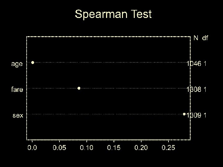
Can use data to determine where to spend DF • Use Spearman’s Rho to test “importance” • Not peeking because we have chosen to include the term in the model regardless of relation to Y • Use more DF for non-linearity
")
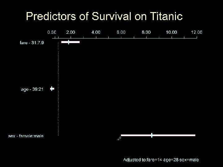
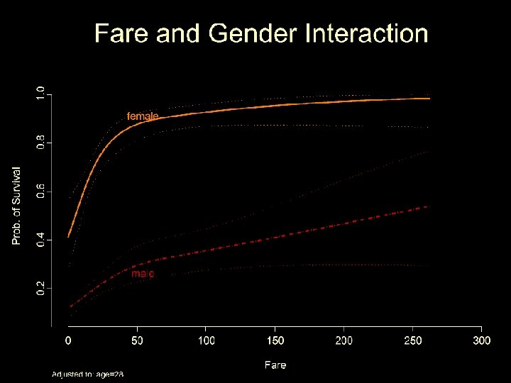
Example-Predict Survival from age, gender, and fare on Titanic: example using S-Plus (or R) software

If you have already decided to include them (and promise to keep them in the model) you can peek at predictors in order to see where to add complexity

Non-linearity using splines
 Y = a + b 1(x<10) + b 2(10<x<20) +")
Linear Spline (piecewise regression) Y = a + b 1(x<10) + b 2(10<x<20) + b 3 (x >20)
 knots")
Cubic Spline (non-linear piecewise regression) knots
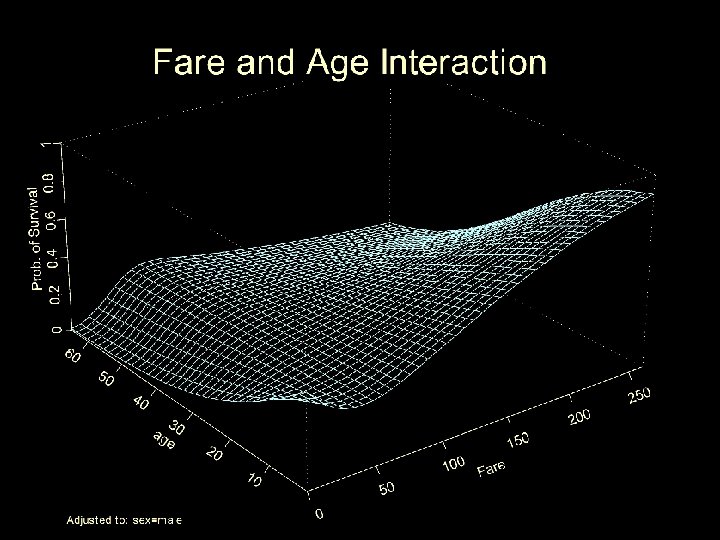
+age+sex)^2, x=T, y=T) anova(fitfare) Spline with 3 knots")
Logistic regression model fitfare<-lrm(survived~(rcs(fare, 3)+age+sex)^2, x=T, y=T) anova(fitfare) Spline with 3 knots
 55. 1")
Wald Statistics Response: survived Factor Chi-Square d. f. fare (Factor+Higher Order Factors) 55. 1 6 All Interactions 13. 8 4 Nonlinear (Factor+Higher Order Factors) 21. 9 3 age (Factor+Higher Order Factors) 22. 2 4 All Interactions 16. 7 3 sex (Factor+Higher Order Factors) 208. 7 4 All Interactions 20. 2 3 fare * age (Factor+Higher Order Factors) 8. 5 2 Nonlinear 8. 5 1 Nonlinear Interaction : f(A, B) vs. AB 8. 5 1 fare * sex (Factor+Higher Order Factors) 6. 4 2 Nonlinear 1. 5 1 Nonlinear Interaction : f(A, B) vs. AB 1. 5 1 age * sex (Factor+Higher Order Factors) 9. 9 1 TOTAL NONLINEAR 21. 9 3 TOTAL INTERACTION 24. 9 5 TOTAL NONLINEAR + INTERACTION 38. 3 6 TOTAL 245. 3 9 P <. 0001 0. 0079 0. 0001 0. 0002 0. 0008 <. 0001 0. 0002 0. 0142 0. 0036 0. 0401 0. 2153 0. 0016 0. 0001 <. 0001

Bootstrap Validation Index Dxy R 2 Intercept Slope Training 0. 6565 0. 4273 0. 0000 1. 0000 Corrected 0. 646 0. 407 -0. 011 0. 952

Summary • Think about your model • Collect enough data

Summary • Measure well • Don’t destroy what you’ve measured

Summary • Pick your variables ahead of time and collect enough data to test the model you want • Keep all your variables in the model unless extremely unimportant

Summary • Use more df on important variables, fewer df on “nuisance” variables • Don’t peek at Y to combine, discard, or transform variables

Summary • Estimate validity and shrinkage with bootstrap

Summary • By all means, tinker with the model later, but be aware of the costs of tinkering • Don’t forget to say you tinkered • Go collect more data

Web links for references, software, and more • Harrell’s regression modeling text – http: //hesweb 1. med. virginia. edu/biostat/rms/ • SAS Macros for spline estimation – http: //hesweb 1. med. virginia. edu/biostat/SAS/survrisk. txt • Some results comparing validation methods – http: //hesweb 1. med. virginia. edu/biostat/reports/logistic. val. pdf • SAS code for bootstrap – ftp: //ftp. sas. com/pub/neural/jackboot. sas • S-Plus home page – insightful. com • Mike Babyak’s e-mail – michael. babyak@duke. edu • This presentation – http: //www. duke. edu/~mbabyak

• www. duke. edu/~mababyak • michael. babyak @ duke. edu • symptomresearch. nih. gov/chapter_8/
- Slides: 90