Building Macro Model Chapter 12 Building the Macro

Building Macro Model Chapter 12

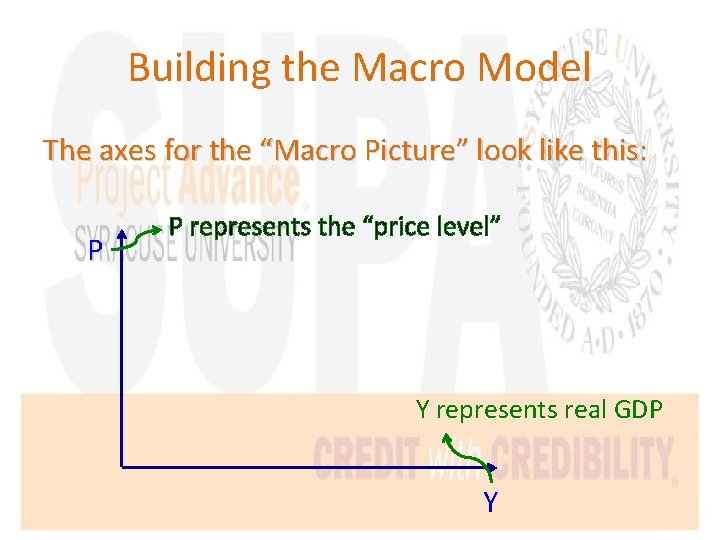
Building the Macro Model The axes for the “Macro Picture” look like this: P P represents the “price level” Y represents real GDP Y

Building the Macro Model We’ll have an orientation point along the Y axis that represents the point at which Y = YF: P YF Y

Building the Macro Model • When the economy is at the Natural Rate (YF) – it’s using its resources most efficiently and effectively … there’s no “slack” – …And we noted the Micro condition that must be true for this to be the Macro case: – General Competitive Equilibrium (GCE)

Building the Macro Model • General Competitive Equilibrium (GCE) is realized when: – “all of the micro adjustments are completed under our nice assumptions” • We’re going to use this expression to define the Macro “Long Run”

Building the Macro Model • The “Long Run” is not measured in time, but rather by process … – In the Long Run “all of the micro adjustments are completed under our nice assumptions” … • So…in the Long Run – the Micro economy will be at GCE and – the Macro Economy will be at YF

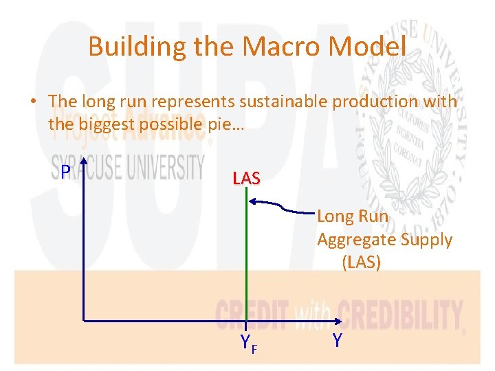
Building the Macro Model • The long run represents sustainable production with the biggest possible pie… P LAS Long Run Aggregate Supply (LAS) YF Y

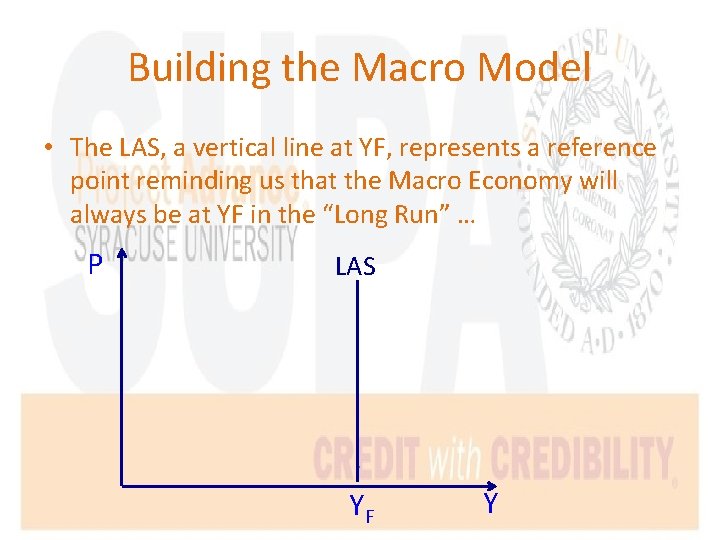
Building the Macro Model • The LAS, a vertical line at YF, represents a reference point reminding us that the Macro Economy will always be at YF in the “Long Run” … P LAS YF Y

Building the Macro Model • In the Long Run “all of the micro adjustments are completed under our nice assumptions” • In the Short Run some of the micro adjustments have not happened – In particular … in the Short Run factor prices are constant

Building the Macro Model • The Short Run Aggregate Supply (AS) line reflects how, given constant factor prices, increasing Y ultimately puts pressure on the economy as it gets closer to or even exceeds YF

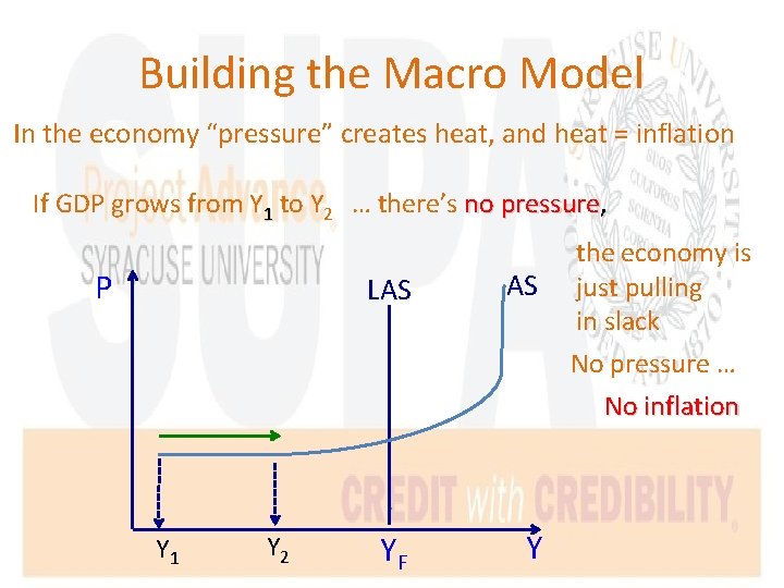
Building the Macro Model In the economy “pressure” creates heat, and heat = inflation If GDP grows from Y 1 to Y 2 … there’s no pressure, P LAS AS the economy is just pulling in slack No pressure … No inflation Y 1 Y 2 YF Y

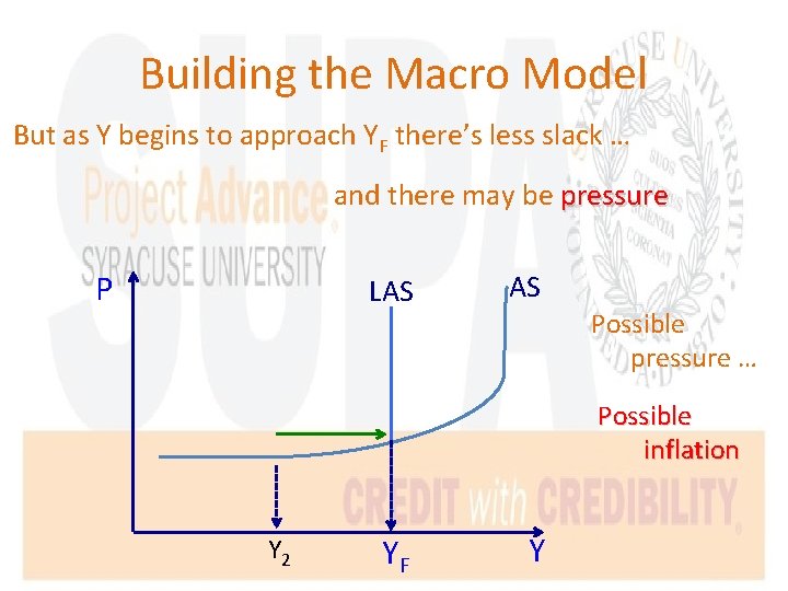
Building the Macro Model But as Y begins to approach YF there’s less slack … and there may be pressure P LAS AS Possible pressure … Possible inflation Y 2 YF Y

Building the Macro Model When Y surpasses YF resources are being stretched that creates pressure … P AS LAS P 1 P 0 and pressure produces heat … Inflation YF Y 3 Y

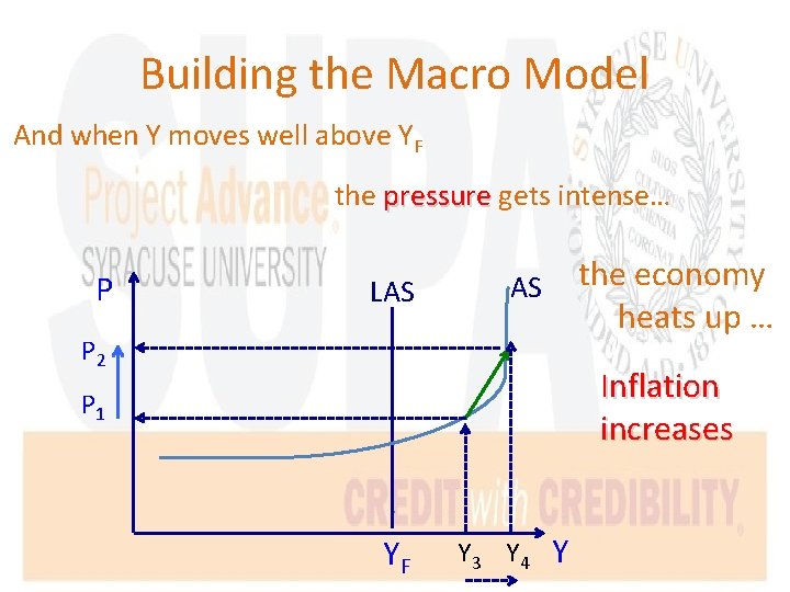
Building the Macro Model And when Y moves well above YF the pressure gets intense… P LAS the economy heats up … AS P 2 Inflation increases P 1 YF Y 3 Y 4 Y

Building the Macro Model • The AS line traces the pressure created by increasing the production of real GDP (Y) • When there’s plenty of slack … no pressure … no problem… • But as we “take in” the slack that can begin to create pressure … that creates a problem: Inflation – If we push the economy beyond full sustainable capacity, YF … inflation can become a serious problem

Building the Macro Model • So if plenty of slack means no problem from pressure (i. e. , no inflation) … plenty of slack is a good thing … right? • NO! – More slack implies more demand deficient unemployment

Building the Macro Model • Less slack implies less demand deficient unemployment … so less slack is a good thing … right? • Not necessarily … less slack raises the danger of inflation • So the challenge of achieving a healthy economy is to eliminate the slack … to get to YF, without setting off inflation

The AS Line

Aggregate Demand What “moves” the economy along the AS line?

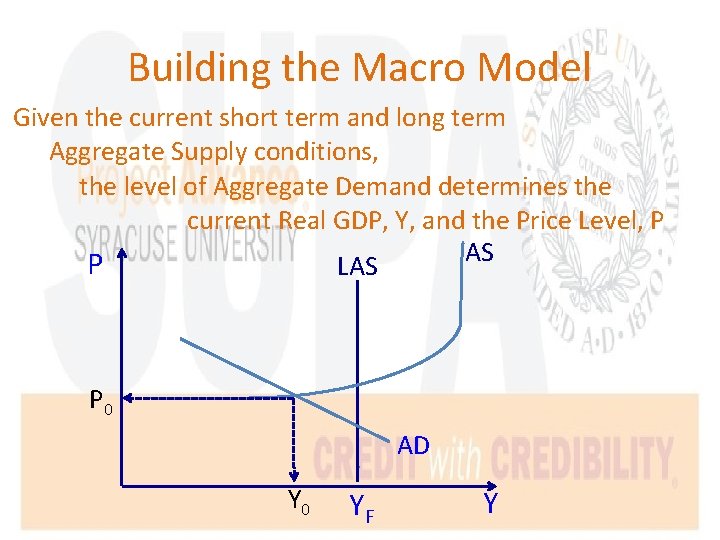
Building the Macro Model Given the current short term and long term Aggregate Supply conditions, the level of Aggregate Demand determines the current Real GDP, Y, and the Price Level, P AS P LAS P 0 AD Y 0 YF Y

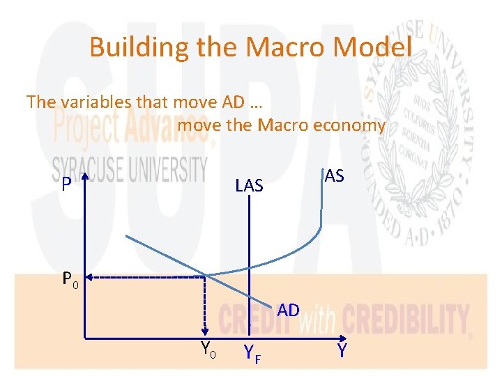
Building the Macro Model The variables that move AD … move the Macro economy P AS LAS P 0 AD Y 0 YF Y

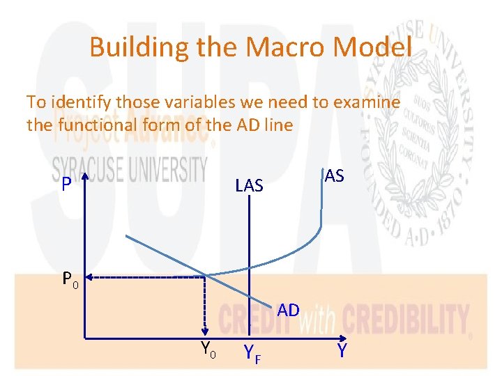
Building the Macro Model To identify those variables we need to examine the functional form of the AD line P AS LAS P 0 AD Y 0 YF Y

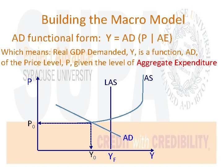
Building the Macro Model AD functional form: Y = AD (P | AE) Which means: Real GDP Demanded, Y, is a function, AD, of the Price Level, P, given the level of Aggregate Expenditure P AS LAS P 0 AD Y 0 YF Y

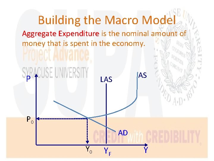
Building the Macro Model Aggregate Expenditure is the nominal amount of money that is spent in the economy. P AS LAS P 0 AD Y 0 YF Y

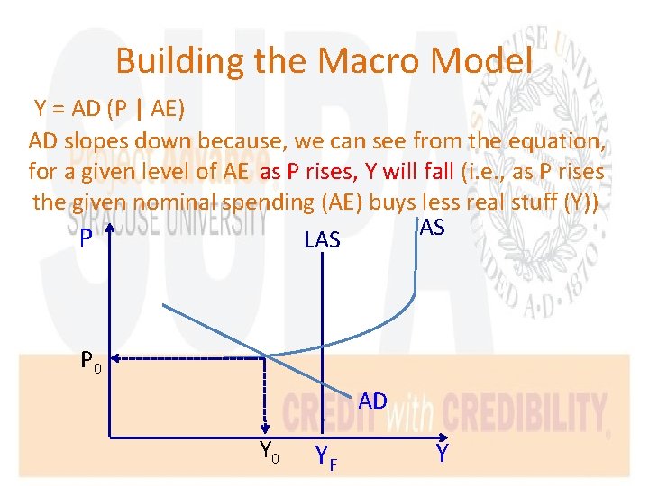
Building the Macro Model Y = AD (P | AE) AD slopes down because, we can see from the equation, for a given level of AE as P rises, Y will fall (i. e. , as P rises the given nominal spending (AE) buys less real stuff (Y)) AS P LAS P 0 AD Y 0 YF Y

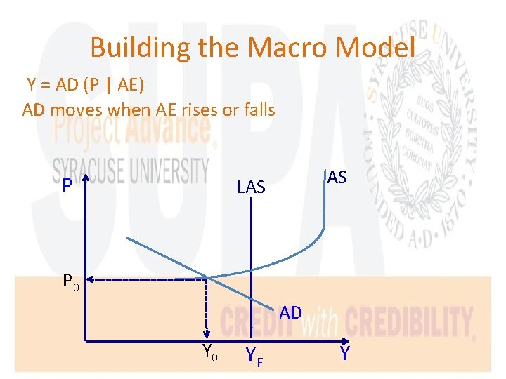
Building the Macro Model Y = AD (P | AE) AD moves when AE rises or falls P AS LAS P 0 AD Y 0 YF Y

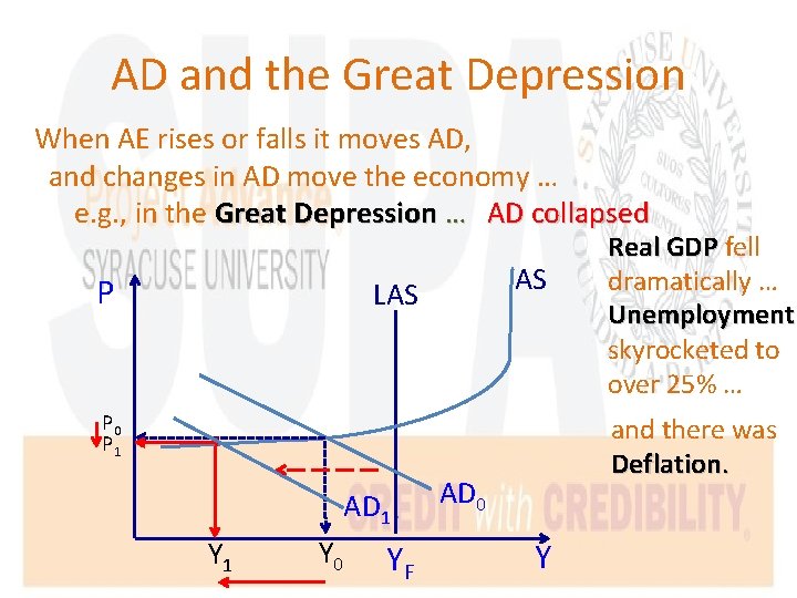
AD and the Great Depression When AE rises or falls it moves AD, and changes in AD move the economy … e. g. , in the Great Depression … AD collapsed P AS LAS P 0 P 1 AD 1 Y 0 YF Real GDP fell dramatically … Unemployment skyrocketed to over 25% … and there was Deflation. AD 0 Y

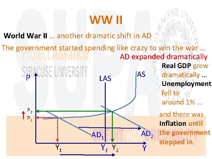
WW II World War II … another dramatic shift in AD The government started spending like crazy to win the war … AD expanded dramatically P LAS AS P 2 P 1 AD 1 YF Y 2 AD 2 Y Real GDP grew dramatically … Unemployment fell to around 1% … and there was Inflation until the government stepped in.

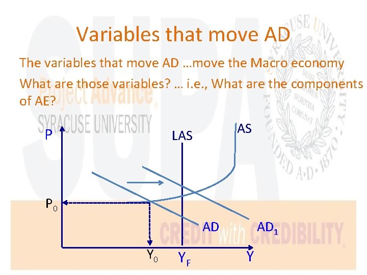
Variables that move AD The variables that move AD …move the Macro economy What are those variables? … i. e. , What are the components of AE? P AS LAS P 0 AD 1 AD Y 0 YF Y

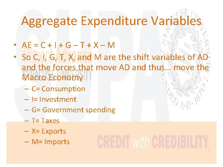
Aggregate Expenditure Variables • AE = C + I + G – T + X – M • So C, I, G, T, X, and M are the shift variables of AD and the forces that move AD and thus… move the Macro Economy – C= Consumption – I= Investment – G= Government spending – T= Taxes – X= Exports – M= Imports

Consumption • Y = AD (P | C, I, G, T, X, and M ) • C is Consumption – The aggregate nominal amount of spending we do as consumers • makes up 65 -70% of AD. – It’s big … but it doesn’t usually change dramatically or quickly. People tend to try and maintain their standard of living

Consumption • Ceteris paribus … • More Consumption is stimulative – It shifts AD right. • Less Consumption is contractionary – It shifts AD left.

Investment • Y = AD (P | C, I, G, T, X, and M ) • I is Investment – The aggregate, nominal amount of spending we do as individuals or firms to increase our production capital or inventories – It is not nearly as big as C, but it is significant and more importantly … it is volatile • It can change dramatically and quickly … driven by the optimism of our “animal spirits” (Keynes) or the fears of our human vulnerability

Investment • Ceteris paribus … • More Investment is stimulative … – It shifts AD right. • Less Investment is contractionary … – It shifts AD left.

Government Spending and Taxes • Y = AD (P | C, I, G, T, X, and M ) • G is Government Spending and T is Taxes – The aggregate nominal spending and taxing the government does. – G and AD move together – the more Government Spending, the more AD, and vice versa – T and AD move in opposite directions – the more Government Taxing, the less AD, and vice versa

Spending, Taxes, and Budget • (G – T) is the Government’s Budget Position – (G – T) = 0 is a Balanced Budget – (G – T) < 0 is a Budget Surplus – (G – T) > 0 is a Budget Deficit

Spending, Taxes, and Budget • Ceteris paribus … • (G – T) = 0 , a Balanced Budget, is neutral. It doesn’t shift AD • (G – T) < 0 , a Budget Surplus, is contractionary. It shifts AD left. • (G – T) > 0 , a Budget Deficit, is stimulative. It shifts AD right.

Exports and Imports • Y = AD (P | C, I, G, T, X, and M ) • X is Exports and M is Imports – X is the aggregate nominal spending on domestic items by foreigners, M is the aggregate nominal spending on foreign items by domestic buyers – X and AD move together – the more foreigners spend domestically, the more AD, and vice versa – M and AD move in opposite directions – the more spent on foreign items the less AD, and vice versa

Exports and Imports • • (X – M) is the Trade Balance (X – M) = 0 is a Balanced Trade (X – M) < 0 is a Trade Deficit (X – M) > 0 is a Trade Surplus

Exports and Imports • Ceteris paribus … • (X – M) = 0 , a Balanced Trade, is neutral. It doesn’t shift AD • (X – M) < 0 , a Trade Deficit, is contractionary. It shifts AD left. • (X – M) > 0 , a Trade Surplus is stimulative. It shifts AD right.

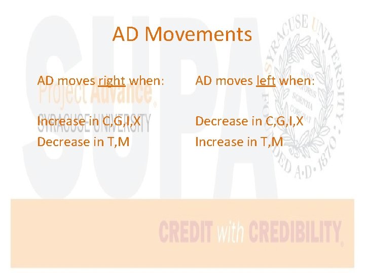
AD Movements AD moves right when: AD moves left when: Increase in C, G, I, X Decrease in T, M Decrease in C, G, I, X Increase in T, M

LAS and AS The Shift Variables

LAS and AS • LAS shift variables – LAS is vertical at YF because it represents the condition of the economy in the Long Run, independent of the Price Level, P

The Long Run • The economy has reached the Long Run when all the micro adjustments are completed under our nice assumptions. • How long is this? – Describe the macro condition in terms of GDP and Unemployment in the Long Run? – What is the micro condition in the Long Run?

The Long Run • The micro condition in the Long Run is GCE. • What did we learn determines the size of the “pie” when the economy is at GCE? • It’s determined by the size of society’s endowment … – So growth in society’s endowment grows the size of the “pie” society can produce

The Long Run • As growth in society’s endowment increases the size of the “pie” society can produce at GCE grows – by definition it is growing the Long Term Macro capacity of the economy… • YF grows, shifting LAS to the right, as society’s resource endowment grows: – Population resource growth – Natural resource growth – Capital resource growth

AS Shift Variables • AS traces the pressure (inflation) created by increasing the production of real GDP (Y), holding factor prices constant – AS reflects the “cost structure” of the macro economy for a given level of factor prices

AS Shift Variables • Anything that raises “cost structure” of the macro economy shifts AS up …because for any level of real GDP (Y), it costs more to make that aggregate output … – so the Price Level, P, at every level of Y rises to cover this higher cost structure

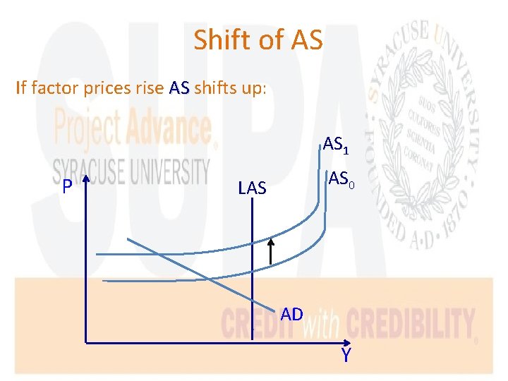
Shift of AS If factor prices rise AS shifts up: AS 1 P AS 0 LAS AD Y

Stagflation • Shifting AS up can result in “stagflation” …inflation and higher unemployment at the same time – This happened during the OPEC oil embargo of the 1970 s

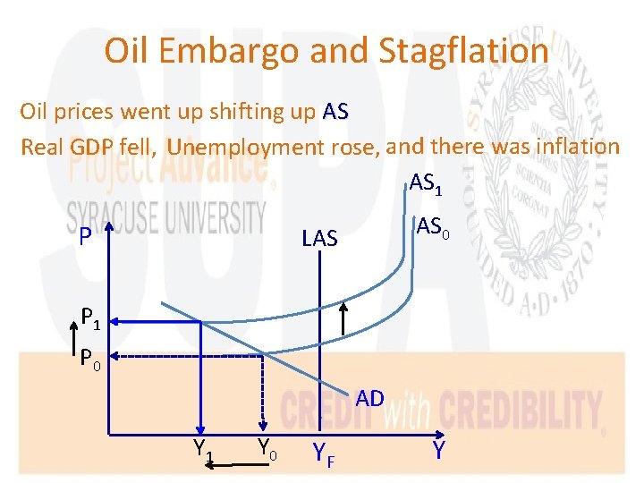
Oil Embargo and Stagflation Oil prices went up shifting up AS Real GDP fell, Unemployment rose, and there was inflation AS 1 P AS 0 LAS P 1 P 0 AD Y 1 Y 0 YF Y

Wage-Price Spiral • Inflation set off by expanding AD sets off a wage response – When wages increase, AS shifts up – If AD continues to shift outward, the net result after several of these is as follows:

Wage-Price Spiral

Macro Model…Summary • LAS shifts right with increases in society’s endowment … this is growth in the economy (It can also shift left…why? ) • AS shifts up and down with changes in factor prices • AD shifts right or left with changes in C, I, G, T, X, & M • Next we explore the sources of the forces that determine the level of C, I, G, T, X, & M