Building Compu Cell 3 D Simulations StepbyStep Tutorial

Building Compu. Cell 3 D Simulations Step-by-Step Tutorial Maciej Swat

Building Your First Compu. Cell 3 D Simulation All simulation parameters are controlled by the config file. The config file allows you to only add those features needed for your current simulation, enabling better use of system resources. Define Lattice and Simulation Parameters Cell < Compu. Cell 3 D> <Potts> <Dimensions x=“ 100" y=“ 100" z=“ 1"/> <Steps>10</Steps> <Temperature>2</Temperature> <Flip 2 Dim. Ratio>1</Flip 2 Dim. Ratio> </Potts> … </Compu. Cell 3 D>

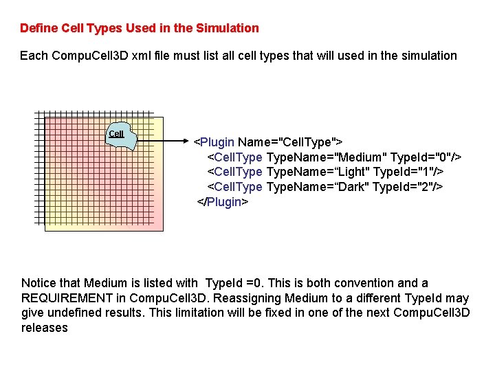
Define Cell Types Used in the Simulation Each Compu. Cell 3 D xml file must list all cell types that will used in the simulation Cell <Plugin Name="Cell. Type"> <Cell. Type. Name="Medium" Type. Id="0"/> <Cell. Type. Name=“Light" Type. Id="1"/> <Cell. Type. Name=“Dark" Type. Id="2"/> </Plugin> Notice that Medium is listed with Type. Id =0. This is both convention and a REQUIREMENT in Compu. Cell 3 D. Reassigning Medium to a different Type. Id may give undefined results. This limitation will be fixed in one of the next Compu. Cell 3 D releases

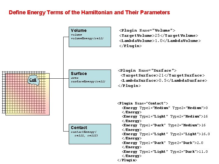
Define Energy Terms of the Hamiltonian and Their Parameters Volume volume. Energy(cell) Surface Cell area surface. Energy(cell) Contact contact. Energy( cell 1, cell 2) <Plugin Name="Volume"> <Target. Volume>25</Target. Volume> <Lambda. Volume>1. 0</Lambda. Volume> </Plugin> <Plugin Name="Surface"> <Target. Surface>21</Target. Surface> <Lambda. Surface>0. 5</Lambda. Surface> </Plugin> <Plugin Name="Contact"> <Energy Type 1="Medium" Type 2="Medium">0 </Energy> <Energy Type 1="Light" Type 2="Medium">16 </Energy> <Energy Type 1="Dark" Type 2="Medium">16 </Energy> <Energy Type 1="Light" Type 2="Light">16. 0 </Energy> <Energy Type 1="Dark" Type 2="Dark">2. 0 </Energy> <Energy Type 1="Light" Type 2="Dark">11. 0 </Energy> </Plugin>

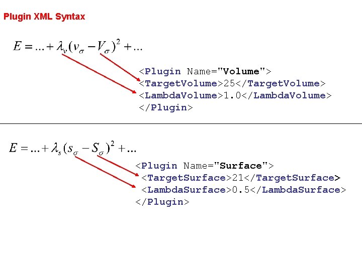
Plugin XML Syntax <Plugin Name="Volume"> <Target. Volume>25</Target. Volume> <Lambda. Volume>1. 0</Lambda. Volume> </Plugin> <Plugin Name="Surface"> <Target. Surface>21</Target. Surface> <Lambda. Surface>0. 5</Lambda. Surface> </Plugin>

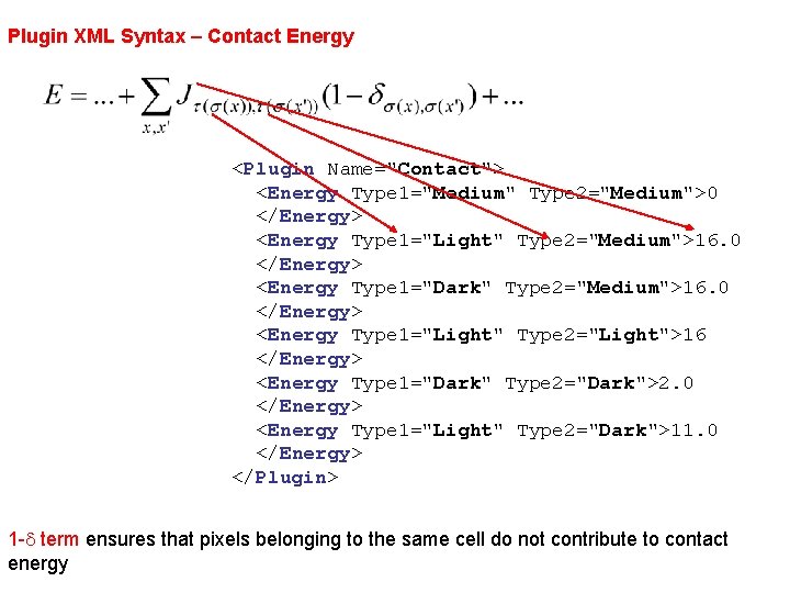
Plugin XML Syntax – Contact Energy <Plugin Name="Contact"> <Energy Type 1="Medium" Type 2="Medium">0 </Energy> <Energy Type 1="Light" Type 2="Medium">16. 0 </Energy> <Energy Type 1="Dark" Type 2="Medium">16. 0 </Energy> <Energy Type 1="Light" Type 2="Light">16 </Energy> <Energy Type 1="Dark" Type 2="Dark">2. 0 </Energy> <Energy Type 1="Light" Type 2="Dark">11. 0 </Energy> </Plugin> 1 -d term ensures that pixels belonging to the same cell do not contribute to contact energy

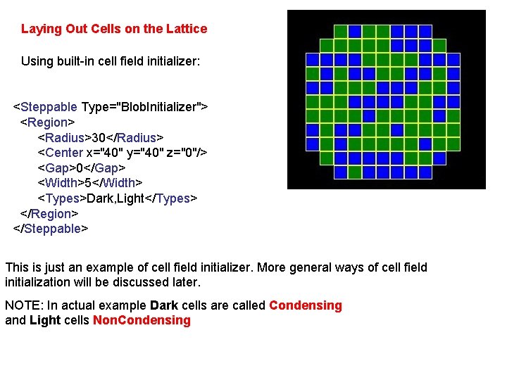
Laying Out Cells on the Lattice Using built-in cell field initializer: <Steppable Type="Blob. Initializer"> <Region> <Radius>30</Radius> <Center x="40" y="40" z="0"/> <Gap>0</Gap> <Width>5</Width> <Types>Dark, Light</Types> </Region> </Steppable> This is just an example of cell field initializer. More general ways of cell field initialization will be discussed later. NOTE: In actual example Dark cells are called Condensing and Light cells Non. Condensing

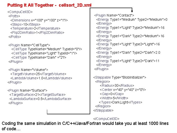
Putting It All Together - cellsort_2 D. xml <Compu. Cell 3 D> <Potts> <Dimensions x="100" y="100" z="1"/> <Steps>10</Steps> <Temperature>2</Temperature> <Flip 2 Dim. Ratio>1</Flip 2 Dim. Ratio> </Potts> <Plugin Name="Cell. Type"> <Cell. Type. Name="Medium" Type. Id="0"/> <Cell. Type. Name=“Light" Type. Id="1"/> <Cell. Type. Name=“Dark" ="2"/> </Plugin> <Plugin Name="Volume"> <Target. Volume>25</Target. Volume> <Lambda. Volume>1. 0</Lambda. Volume> </Plugin> <Plugin Name="Surface"> <Target. Surface>21</Target. Surface> <Lambda. Surface>0. 5</Lambda. Surface> </Plugin> <Plugin Name="Contact"> <Energy Type 1="Medium" Type 2="Medium">0 </Energy> <Energy Type 1="Light" Type 2="Medium">16 </Energy> <Energy Type 1="Dark" Type 2="Medium">16 </Energy> <Energy Type 1="Light" Type 2="Light">16 </Energy> <Energy Type 1="Dark" Type 2="Dark">2. 0 </Energy> <Energy Type 1="Light" Type 2="Dark">11 </Energy> </Plugin> <Steppable Type="Blob. Initializer"> <Region> <Radius>30</Radius> <Center x="40" y="40" z="0"/> <Gap>0</Gap> <Width>5</Width> <Types>Dark, Light</Types> </Region> </Steppable> </Compu. Cell 3 D> Coding the same simulation in C/C++/Java/Fortran would take you at least 1000 lines of code…

Putting It All Together - Avoiding Common Errors in XML code 1. First specify Potts section, then list all the plugins and finally list all the steppables. This is the correct order and if you mix e. g. plugins with steppables you will get an error. Remember the correct order is • Potts • Plugins • Steppables 2. Remember to match every xml tag with a closing tag <Plugin> … </Plugin> 3. Watch for typos – if there is an error in the XML syntax CC 3 D will give you an error pointing to the location of an offending line 4. Modify/reuse available examples rather than starting from scratch – saves a lot of time

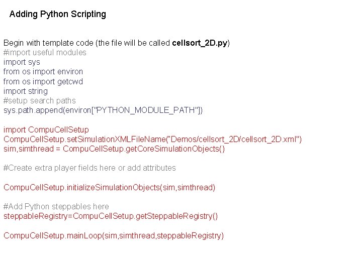
Adding Python Scripting Begin with template code (the file will be called cellsort_2 D. py) #import useful modules import sys from os import environ from os import getcwd import string #setup search paths sys. path. append(environ["PYTHON_MODULE_PATH"]) import Compu. Cell. Setup. set. Simulation. XMLFile. Name(“Demos/cellsort_2 D. xml") sim, simthread = Compu. Cell. Setup. get. Core. Simulation. Objects() #Create extra player fields here or add attributes Compu. Cell. Setup. initialize. Simulation. Objects(sim, simthread) #Add Python steppables here steppable. Registry=Compu. Cell. Setup. get. Steppable. Registry() Compu. Cell. Setup. main. Loop(sim, simthread, steppable. Registry)

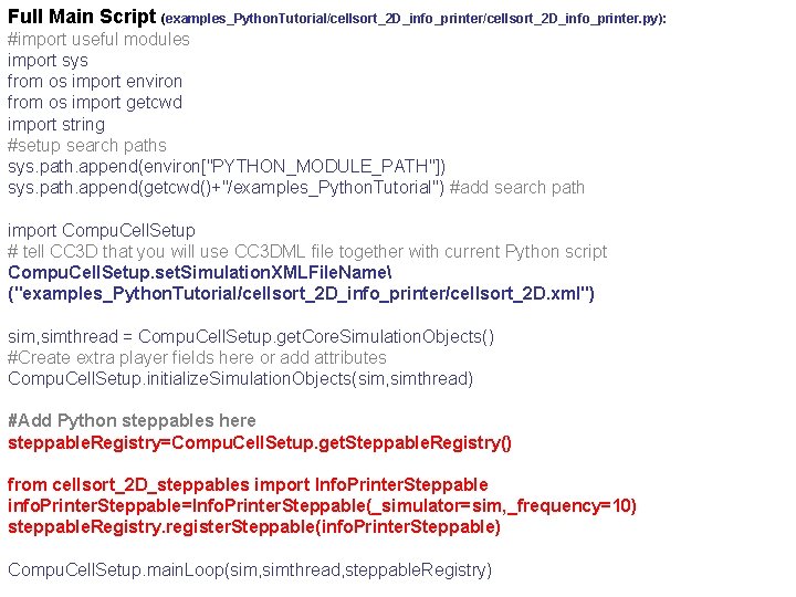
Full Main Script (examples_Python. Tutorial/cellsort_2 D_info_printer. py): #import useful modules import sys from os import environ from os import getcwd import string #setup search paths sys. path. append(environ["PYTHON_MODULE_PATH"]) sys. path. append(getcwd()+"/examples_Python. Tutorial") #add search path import Compu. Cell. Setup # tell CC 3 D that you will use CC 3 DML file together with current Python script Compu. Cell. Setup. set. Simulation. XMLFile. Name ("examples_Python. Tutorial/cellsort_2 D_info_printer/cellsort_2 D. xml") sim, simthread = Compu. Cell. Setup. get. Core. Simulation. Objects() #Create extra player fields here or add attributes Compu. Cell. Setup. initialize. Simulation. Objects(sim, simthread) #Add Python steppables here steppable. Registry=Compu. Cell. Setup. get. Steppable. Registry() from cellsort_2 D_steppables import Info. Printer. Steppable info. Printer. Steppable=Info. Printer. Steppable(_simulator=sim, _frequency=10) steppable. Registry. register. Steppable(info. Printer. Steppable) Compu. Cell. Setup. main. Loop(sim, simthread, steppable. Registry)

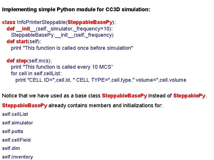
Implementing simple Python module for CC 3 D simulation: class Info. Printer. Steppable(Steppable. Base. Py): def __init__(self, _simulator, _frequency=10): Steppable. Base. Py. __init__(self, _frequency) def start(self): print "This function is called once before simulation" def step(self, mcs): print "This function is called every 10 MCS“ for cell in self. cell. List: print "CELL ID=", cell. id, " CELL TYPE=", cell. type, " volume=", cell. volume Notice that we have used as a base class Steppable. Base. Py instead of Steppable. Py. Steppable. Base. Py already contains members and initializations for: self. cell. List self. simulator self. potts self. cell. Field self. dim self. inventory

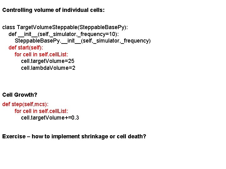
Controlling volume of individual cells: class Target. Volume. Steppable(Steppable. Base. Py): def __init__(self, _simulator, _frequency=10): Steppable. Base. Py. __init__(self, _simulator, _frequency) def start(self): for cell in self. cell. List: cell. target. Volume=25 cell. lambda. Volume=2 Cell Growth? def step(self, mcs): for cell in self. cell. List: cell. target. Volume+=0. 3 Exercise – how to implement shrinkage or cell death?

Mitosis in Compu. Cell 3 D simulations Supporting cell division (mitosis) in Compu. Cell 3 D simulations is a prerequisite for building faithful biomedical simulations. You can use mitosis module (Mitosis Plugin) directly from XML however, its use will be very limited because of the following fact: After cell division you end up with two cells. What parameters should those two cells have (type, target volume etc. )? How do you modify the parameters? The best solution is to manage mitosis from Python and the example below will explain you how to do it. There are two ways to implement mitosis – as a plugin or as a steppable. On older versions we have used plugin-based approach as this was the only option. However steppable based approach is much simpler to implement and we will focus on it first.

import sys from os import environ from os import getcwd import string sys. path. append(environ["PYTHON_MODULE_PATH"]) import Compu. Cell. Setup sim, simthread = Compu. Cell. Setup. get. Core. Simulation. Objects() #add additional attributes py. Attribute. Adder, list. Adder=Compu. Cell. Setup. attach. List. To. Cells(sim) Compu. Cell. Setup. initialize. Simulation. Objects(sim, simthread) import Compu. Cell #notice importing Compu. Cell to main script has to be done after call to get. Core. Simulation. Objects() #Add Python steppables here steppable. Registry=Compu. Cell. Setup. get. Steppable. Registry() from cellsort_2 D_field_modules import Volume. Constraint. Steppable volume. Constraint=Volume. Constraint. Steppable(sim) steppable. Registry. register. Steppable(volume. Constraint) from cellsort_2 D_field_modules import Mitosis. Steppable mitosis. Steppable=Mitosis. Steppable(sim, 1) steppable. Registry. register. Steppable(mitosis. Steppable) Compu. Cell. Setup. main. Loop(sim, simthread, steppable. Registry)

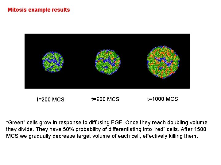
Mitosis example results t=200 MCS t=600 MCS t=1000 MCS “Green” cells grow in response to diffusing FGF. Once they reach doubling volume they divide. They have 50% probability of differentiating into “red” cells. After 1500 MCS we gradually decrease target volume of each cell, effectively killing them.

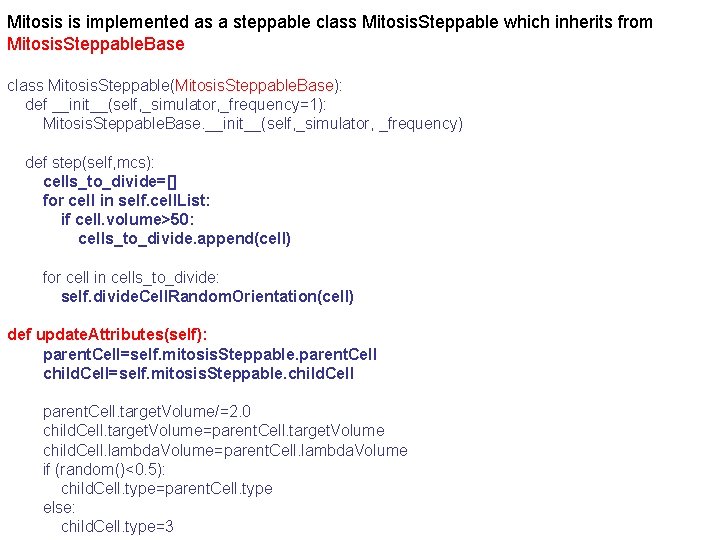
Mitosis is implemented as a steppable class Mitosis. Steppable which inherits from Mitosis. Steppable. Base class Mitosis. Steppable(Mitosis. Steppable. Base): def __init__(self, _simulator, _frequency=1): Mitosis. Steppable. Base. __init__(self, _simulator, _frequency) def step(self, mcs): cells_to_divide=[] for cell in self. cell. List: if cell. volume>50: cells_to_divide. append(cell) for cell in cells_to_divide: self. divide. Cell. Random. Orientation(cell) def update. Attributes(self): parent. Cell=self. mitosis. Steppable. parent. Cell child. Cell=self. mitosis. Steppable. child. Cell parent. Cell. target. Volume/=2. 0 child. Cell. target. Volume=parent. Cell. target. Volume child. Cell. lambda. Volume=parent. Cell. lambda. Volume if (random()<0. 5): child. Cell. type=parent. Cell. type else: child. Cell. type=3

Keeping track of mitotic history of cells – you may skip this during first reading In Compu. Cell 3 D simulations each cell by default will have several attributes such as volume, surface, centroids , target volume, cell id etc. One can write a plugin that attaches additional attributes to a cell during run time. Doing so avoids recompilation of entire Compu. Cell 3 D but requires to write and compile the C++ plugin. It is by far the easiest to attach additional cell attribute in Python. Not only there is no need to recompile anything, but the actual task takes one line of code: py. Attribute. Adder, list. Adder=Compu. Cell. Setup. attach. List. To. Cells(sim) Above we told Compu. Cell 3 D to attach a Python list to each cell that will be produced by the Compu. Cell 3 D kernel. We can access this list very easily from Python level. Python list is dynamic data structure that can grow or shrink and can hold arbitrary Python objects. Therefore by attaching a list to each cell we effectively came up with a way to attach any cell attribute. We may also attach dictionary instead of the list: py. Attribute. Adder, dict. Adder=Compu. Cell. Setup. attach. Dictionary. To. Cells(sim) And everything takes place during run time…

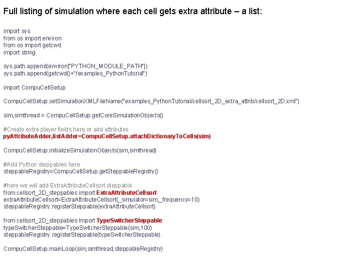
Full listing of simulation where each cell gets extra attribute – a list: import sys from os import environ from os import getcwd import string sys. path. append(environ["PYTHON_MODULE_PATH"]) sys. path. append(getcwd()+"/examples_Python. Tutorial") import Compu. Cell. Setup. set. Simulation. XMLFile. Name("examples_Python. Tutorial/cellsort_2 D_extra_attrib/cellsort_2 D. xml") sim, simthread = Compu. Cell. Setup. get. Core. Simulation. Objects() #Create extra player fields here or add attributes py. Attribute. Adder, list. Adder=Compu. Cell. Setup. attach. Dictionary. To. Cells(sim) Compu. Cell. Setup. initialize. Simulation. Objects(sim, simthread) #Add Python steppables here steppable. Registry=Compu. Cell. Setup. get. Steppable. Registry() #here we will add Extra. Attribute. Cellsort steppable from cellsort_2 D_steppables import Extra. Attribute. Cellsort extra. Attribute. Cellsort=Extra. Attribute. Cellsort(_simulator=sim, _frequency=10) steppable. Registry. register. Steppable(extra. Attribute. Cellsort) from cellsort_2 D_steppables import Type. Switcher. Steppable type. Switcher. Steppable=Type. Switcher. Steppable(sim, 100) steppable. Registry. register. Steppable(type. Switcher. Steppable) Compu. Cell. Setup. main. Loop(sim, simthread, steppable. Registry)

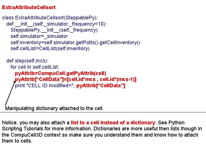
Extra. Attribute. Cellsort class Extra. Attribute. Cellsort(Steppable. Py): def __init__(self, _simulator, _frequency=10): Steppable. Py. __init__(self, _frequency) self. simulator=_simulator self. inventory=self. simulator. get. Potts(). get. Cell. Inventory() self. cell. List=Cell. List(self. inventory) def step(self, mcs): for cell in self. cell. List: py. Attrib=Compu. Cell. get. Py. Attrib(cell) py. Attrib[“Cell. Data”]=[cell. id*mcs , cell. id*(mcs-1)] print "CELL ID modified=", py. Attrib[“Cell. Data”] Manipulating dictionary attached to the cell Notice, you may also attach a list to a cell instead of a dictionary. See Python Scripting Tutorials for more information. Dictionaries are more useful then lists though in the Compu. Cell 3 D context so make sure you understand them and know how to attach them to cells.

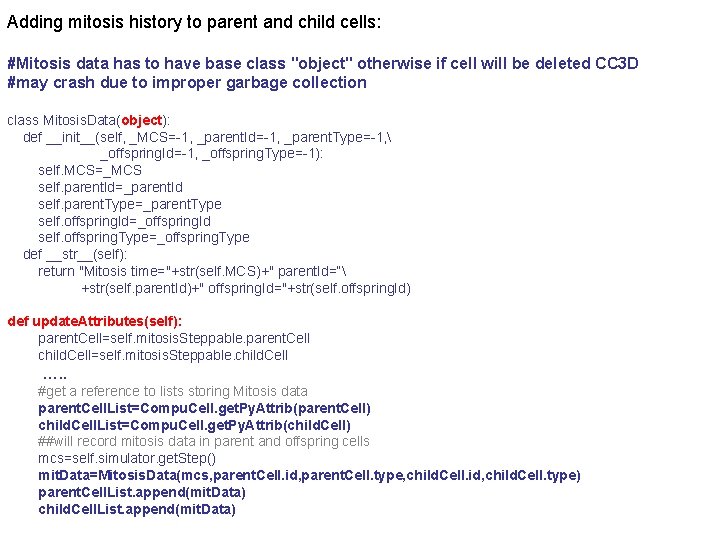
Adding mitosis history to parent and child cells: #Mitosis data has to have base class "object" otherwise if cell will be deleted CC 3 D #may crash due to improper garbage collection class Mitosis. Data(object): def __init__(self, _MCS=-1, _parent. Id=-1, _parent. Type=-1, _offspring. Id=-1, _offspring. Type=-1): self. MCS=_MCS self. parent. Id=_parent. Id self. parent. Type=_parent. Type self. offspring. Id=_offspring. Id self. offspring. Type=_offspring. Type def __str__(self): return "Mitosis time="+str(self. MCS)+" parent. Id=“ +str(self. parent. Id)+" offspring. Id="+str(self. offspring. Id) def update. Attributes(self): parent. Cell=self. mitosis. Steppable. parent. Cell child. Cell=self. mitosis. Steppable. child. Cell …. . #get a reference to lists storing Mitosis data parent. Cell. List=Compu. Cell. get. Py. Attrib(parent. Cell) child. Cell. List=Compu. Cell. get. Py. Attrib(child. Cell) ##will record mitosis data in parent and offspring cells mcs=self. simulator. get. Step() mit. Data=Mitosis. Data(mcs, parent. Cell. id, parent. Cell. type, child. Cell. id, child. Cell. type) parent. Cell. List. append(mit. Data) child. Cell. List. append(mit. Data)

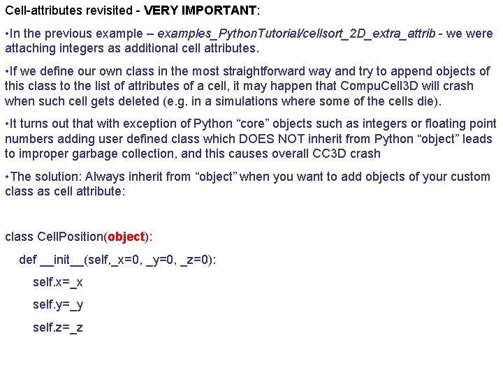
Cell-attributes revisited - VERY IMPORTANT: • In the previous example – examples_Python. Tutorial/cellsort_2 D_extra_attrib - we were attaching integers as additional cell attributes. • If we define our own class in the most straightforward way and try to append objects of this class to the list of attributes of a cell, it may happen that Compu. Cell 3 D will crash when such cell gets deleted (e. g. in a simulations where some of the cells die). • It turns out that with exception of Python “core” objects such as integers or floating point numbers adding user defined class which DOES NOT inherit from Python “object” leads to improper garbage collection, and this causes overall CC 3 D crash • The solution: Always inherit from “object” when you want to add objects of your custom class as cell attribute: class Cell. Position(object): def __init__(self, _x=0, _y=0, _z=0): self. x=_x self. y=_y self. z=_z

Directional Mitosis So far we have divided cells using randomly chosen division axis/plane: class Mitosis. Steppable(Mitosis. Steppable. Base): ……. def step(self, mcs): cells_to_divide=[] for cell in self. cell. List: if cell. volume>50: cells_to_divide. append(cell) for cell in cells_to_divide: self. divide. Cell. Random. Orientation(cell) However Mitosis. Steppable. Base, and consequently any class which inherits from Mitosis. Steppable. Base, allows additional modes of division: • Along major axis/plane of a cell • Along minor axis/plane of a cell • Along user specified axis/plane of the cell

By changing one function name in the Mitosis Steppable we can cause cells to divide along e. g. Major axis: class Mitosis. Steppable(Mitosis. Steppable. Base): def __init__(self, _simulator, _frequency=1): Mitosis. Steppable. Base. __init__(self, _simulator, _frequency) def step(self, mcs): cells_to_divide=[] for cell in self. cell. List: if cell. volume>50: cells_to_divide. append(cell) for cell in cells_to_divide: self. divide. Cell. Along. Major. Axis(cell) # self. divide. Cell. Orientation. Vector. Based(cell, 1, 1, 0) # self. divide. Cell. Along. Major. Axis(cell) Commented lines show addition options in choosing orientation of division axis. Notice that when specifying user-defined orientation we simply specify vector along which the division will take place. The vector does not have to be normalized

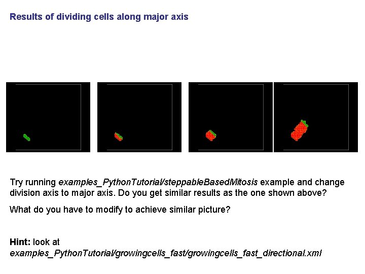
Results of dividing cells along major axis Try running examples_Python. Tutorial/steppable. Based. Mitosis example and change division axis to major axis. Do you get similar results as the one shown above? What do you have to modify to achieve similar picture? Hint: look at examples_Python. Tutorial/growingcells_fast_directional. xml

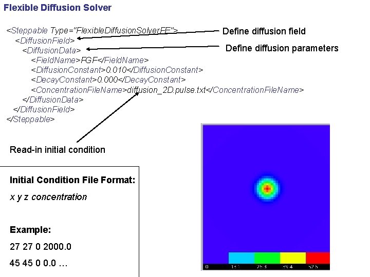
Flexible Diffusion Solver <Steppable Type="Flexible. Diffusion. Solver. FE"> Define diffusion field <Diffusion. Field> Define diffusion parameters <Diffusion. Data> <Field. Name>FGF</Field. Name> <Diffusion. Constant>0. 010</Diffusion. Constant> <Decay. Constant>0. 000</Decay. Constant> <Concentration. File. Name>diffusion_2 D. pulse. txt</Concentration. File. Name> </Diffusion. Data> </Diffusion. Field> </Steppable> Read-in initial condition Initial Condition File Format: x y z concentration Example: 27 27 0 2000. 0 45 45 0 0. 0 …

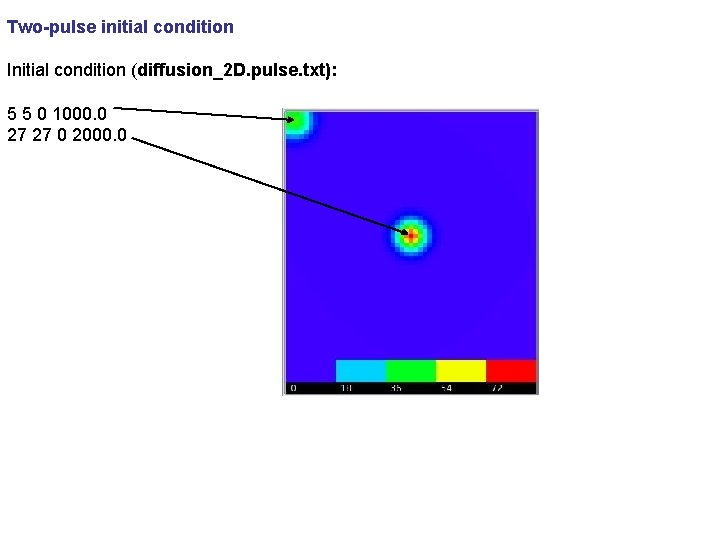
Two-pulse initial condition Initial condition (diffusion_2 D. pulse. txt): 5 5 0 1000. 0 27 27 0 2000. 0

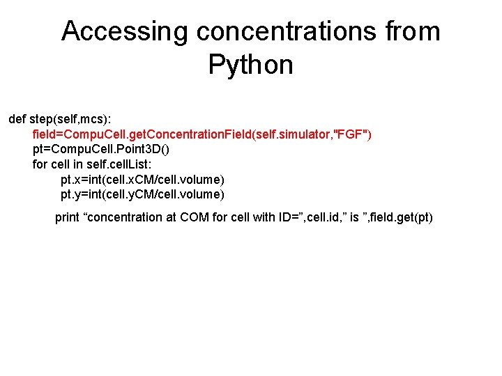
Accessing concentrations from Python def step(self, mcs): field=Compu. Cell. get. Concentration. Field(self. simulator, "FGF") pt=Compu. Cell. Point 3 D() for cell in self. cell. List: pt. x=int(cell. x. CM/cell. volume) pt. y=int(cell. y. CM/cell. volume) print “concentration at COM for cell with ID=”, cell. id, ” is ”, field. get(pt)

Putting things together • By combining cell growth, concentration fields, mitosis, cell type differentiation you can start building biologically interesting simulations. • Adding more “ingredients” to simulations does not require any more knowledge. All you have to know is how to copy, paste, and modify code snippets.

Linking SBML models to describe cell properties • Specifying cell properties individually is quite straight forward but better approach is to use underlying molecular model to control cell bohavior. • Use soslib Python wrapper developed by Ryan Roper (UW) • Final release is pending

Molecular Circuits Inside Each Cell • Define molecular pathway model in Jarnac (or if you prefer any other tool which exports SBML) • Save pathway model in SBML format • Load SBML model to each Compu. Cell 3 D cell • Solve SBML model • Make cell properties of cell depend on the current state of the SBML model

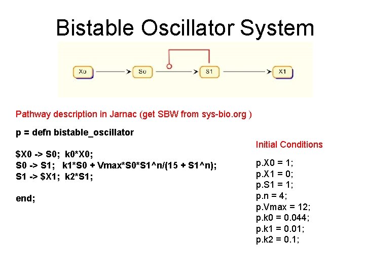
Bistable Oscillator System Pathway description in Jarnac (get SBW from sys-bio. org ) p = defn bistable_oscillator $X 0 -> S 0; k 0*X 0; S 0 -> S 1; k 1*S 0 + Vmax*S 0*S 1^n/(15 + S 1^n); S 1 -> $X 1; k 2*S 1; end; Initial Conditions p. X 0 = 1; p. X 1 = 0; p. S 1 = 1; p. n = 4; p. Vmax = 12; p. k 0 = 0. 044; p. k 1 = 0. 01; p. k 2 = 0. 1;

Controling cell-cell adhesion using molecular toy circuit • Inside each cell we run (i. e. solve) reaction kinetics model – specified in SBML format • We extract concentration of molecular species to control cell-cell adhesion • We may conveniently plot time series of species concentration in CC 3 D